Day By Day
Notes for MATH 206
Fall 2008
Activity: Go over syllabus. Take roll. Functions activities.
Goals: Review course objectives: collect data, summarize information, and make inferences.
I have divided this course into three "units". Unit 1 (Days 1 through 8) is about basic functions. Unit 2 (Days 9 through 17) is about derivatives and their uses. Unit 3 (Days 18 through 28) is about integration and multi-variable functions.
I believe to be successful in this course, you must READ the text carefully, working many practice problems. Our activities in class will sometimes be unrelated to the homework you practice and/or turn in for the homework portion of your grade; instead they will be for understanding of the underlying principles. For example, on Day 9 you will draw sample graphs and derivatives, then try to reconstruct the original graph. This is something you would never do in practice, but which I think will demonstrate several lessons for us. In these notes, I will try to point out to you when we're doing something to gain understanding, and when we're doing something to gain skills.
Each semester, I am disappointed with the small number of students who come to me for help outside of class. I suspect some of you are embarrassed to seek help, or you may feel I will think less of you for not "getting it" on your own. Personally, I think that if you are struggling and cannot make sense of what we are doing, and don't seek help, you are cheating yourself out of your own education. I am here to help you learn mathematics. Please ask questions when you have them; there is no such thing as a stupid question. Often other students have the same questions but are also too shy to ask them in class. If you are still too shy to ask questions in class, come to my office hours or make an appointment.
I believe you get out of something what you put into it. Very rarely will someone fail a class by attending every day, doing all the assignments, and working many practice problems; typically people fail by not applying themselves enough - either through missing classes, or by not allocating enough time for the material. Obviously I cannot tell you how much time to spend each week on this class; you must all find the right balance for you and your life's priorities. One last piece of advice: don't procrastinate. I believe mathematics is learned best by daily exposure. Cramming for exams may get you a passing grade, but you are only cheating yourself out of understanding and learning.
Today we will begin by discussing functions. Quite simply, a function is a rule. From an input value, a function gives the output value. The set of possible inputs is called the domain, and the set of output values is called the range. The input value is sometimes called the independent value, and the output value the dependent value. One of the chief goals of mathematics is to model real world phenomena with functions. Therefore it is important for us to be familiar with their uses and roles.
Throughout the course, we will try to look at functions from four different viewpoints. Data will be presented to us in tabular form, graphical form, algebraic form, or verbally. It will be up to us to determine the most appropriate method of describing the function. A common misconception that I hope to dispel is that equations are synonymous with functions. Equations are only one method of describing functions. Our text makes an honest effort to display functions for us in all four forms.
Today I would like to explore functions graphically, verbally, and algebraically. We will begin with a discussion of a hypothetical flight between two cities. Then I will have you work in groups on three projects.
In these notes, I will put the daily task in gray background.
I have three activities for us to become more familiar with functions.
Activity 1:
Graphical and Verbal Description.
The value of a car goes down as the car gets older, so we can think of the value of a car, V, in thousands of dollars, as a function of the age of a car, a, in years. We have V = f(a).
1) Draw a possible graph of V against a. You don't need scales on the axes, but label each axis as V or a.
2) What does the statement f(5) = 6 tell you about the value of the car? Be sure to use units for 5 and for 6. Label this as a point on your graph, and mark the 5 and the 6 on the appropriate axes.
3) Put a vertical intercept of 15 on your graph of the function. Explain the meaning of this vertical intercept in terms of the value of the car.
4) Put a horizontal intercept of 10 on your graph of the function. Explain the meaning of this horizontal intercept in terms of the value of the car.
Activity 2:
Algebraic and Verbal Description.
From a length of string, form two geometric shapes, a circle and a square. Your goal is to create the smallest area possible.
Activity 3:
Graphical and Algebraic Description.
With our calculators, we have the tools available to explore limits. Specifically, we can hone our intuition about this important topic in calculus.
1) Calculate ![]() for n = 1, 10, 100, 1000, etc.
What seems to be happening?
Can you explain it intuitively?
for n = 1, 10, 100, 1000, etc.
What seems to be happening?
Can you explain it intuitively?
2) Calculate ![]() for n = 1, 10, 100, 1000, etc.
What seems to be happening?
Can you explain it intuitively?
This limit we see here is a very important limit in calculus and
mathematics. We will encounter it
and study it in more detail later.
for n = 1, 10, 100, 1000, etc.
What seems to be happening?
Can you explain it intuitively?
This limit we see here is a very important limit in calculus and
mathematics. We will encounter it
and study it in more detail later.
3) Consider this series: 1, 1/2, 1/3, 1/4, etc. Add successive terms to get a new series of partial sums. That is, find 1, 1+1/2, 1+1/2+1/3, 1+1/2+1/3+1/4, etc. What seems to be happening to this sum? Can you explain it intuitively?
4) Now try this series and repeat what you did in problem 3). 1/2, 1/4, 1/8, 1/16, 1/32, etc. (These are successively smaller powers of two.) What seems to be happening to this sum? Can you explain it intuitively?
5) Using ![]() ,
find the limits as you approach x = 2
from the right and left.
(Approaching from the right means using values just above 2 and
approaching from the left means using values just below 2.) Also find the value right at x = 2.
,
find the limits as you approach x = 2
from the right and left.
(Approaching from the right means using values just above 2 and
approaching from the left means using values just below 2.) Also find the value right at x = 2.
6) Repeat 5) using ![]() .
.
In these notes, I will put sections of computer commands in boxes, like this one. I'm actually hoping that you already are quite familiar with this machine, having already taken MBA I. In these notes, I refer to the calculator as the TI-83. The same commands apply to the TI-84.
Y = is found on the top row of buttons, on the left. You enter equations into whichever Y-variable you want to use. Be careful to enter what you want, that is, pay attention to parentheses, typos, etc! Each Y-variable whose = sign is highlighted will be graphed when the GRAPH button is pressed. In addition, if any plots at the top of the display are highlighted, those too will be plotted, whether you intended them to be or not!
GRAPH is found on the top row of buttons, on the right. This button toggles between the data / numerical entry screens and the graphing window. To leave the graphing window, press any key, or press QUIT, (found by pressing 2nd MODE).
WINDOW is found on the top row of buttons, second from the left. This opens the windows setting screen, which tells you the dimensions and characteristics of the current graphing window. We will mostly change only 4 items: Xmin, Xmax, Ymin, and Ymax. If you like, you may tinker with the other settings.
TRACE is on the top row of buttons, second from the right. This key puts a cursor on the graphing window on one of your y-variables / functions. You may push right and left arrow to move sideways on the selected curve, or up and down arrow to select other curves (if you have entered more than one y-variable.) Be careful: TRACE is dependent on the current window settings. If you need precise values, after pressing TRACE, type the x-value you need evaluated. TRACE will calculate the functional value exactly.
ZoomFit (Zoom 0) Many times, you do not know which is the best viewing window. If you first specify the horizontal endpoints in the WINDOW settings screen (Xmax and Xmin), then you can press ZoomFit (under ZOOM menu, item 0) to have the calculator find the appropriate Ymin and Ymax values. This function is quite handy; I use it a lot myself.
ZStandard (Zoom 6) If you are in love with the numbers between –10 and +10, you should use ZStandard in the ZOOM menu. Otherwise, you may find this key useless!
Goals: (In
these notes, I will summarize each day's activity with a statement of goals for
the day.)
Appreciate the dynamics of collaboration. Understand the different problem solving strategies. Explore some basic limits.
Skills: (In
these notes, each day I will identify skills I believe you should have after working the day's
activity, reading the appropriate sections of the text, and practicing
exercises in the text.
•
Use the "Guess and Check" method of problem solving. This
technique is the essence of the scientific method. There is nothing bad about guessing in order to learn. The better guessers, of course, tend to
get quicker results, but if you have appropriate tools to evaluate your
guesses, then even poor guesses can be refined adequately. By the way, your calculator in this
class will essentially use this 'guess and check' method to 'solve'
equations. It's just that your
calculator works a bit faster than you can. Another related idea is using test numbers to start a
process. That is, perhaps making
up a sample situation will help you 'see' what is going on. I encourage you to use this approach
often; it is the most basic lesson my advisor taught me in graduate
school. He used to say, "Start
with a simple example." That often
meant assuming some specific values for some variables, and working from there
to understand the problem at hand.
•
Physical modeling.
Many times being stuck on a real
world problem can be alleviated by modeling the situation with physical items
or by other simulations. Of course
many situations are infeasible; you can't fly airplanes to simulate scheduling
airline routes, but you can use appropriate diagrams or tokens representing airplanes. Sometimes actually physically representing
something will get you over that 'mental block'.
•
Collaboration.
One of the biggest problems I see
semester after semester with math students is their reluctance to talk about
their math frustration. Talk about things with each other! If you are too timid to talk to me, (or
if you have other reasons for not wanting to chat with me) at least talk to
your peers. Sometimes simply
saying something out loud will open up doors you might not have otherwise opened,
or an offhand remark may inspire someone else's imagination. Of course this doesn't mean that one
person in a group of problem solvers should do all the work; but even if only
one group member 'gets' a solution, the sharing is beneficial to all concerned. The sharer gets to really learn the concept as he/she is forced to explain it; the others get to see a solution they missed.
•
Evaluate limits numerically and graphically. By
using numbers closer and closer to the value in question, whether it is finite
or infinite, your calculator or computer can help you to evaluate limits. There is a caution, however: you must
still use your analytic skills to avoid being fooled. You may have observed this in Exercise 2 of Activity 3. Some limits are easy to evaluate
(simply plug in and evaluate) while others are more complicated (the partial
sums we saw in Exercises 3 and 4 of Activity 3 are often quite difficult to
evaluate or to even decide if they converge.) One of the "big ideas" in calculus is differentiation, and
we need to be comfortable with limits to understand derivatives. Another of the "big ideas" in calculus
is integration, and we need to understand limits such as partial sums to
understand integrals.
•
Recognize the harmonic series. Even though terms in a
series may be getting smaller and smaller, their partial sums may not converge
to a finite number. The sequence
in Exercise 3 of Activity 3 above is called the harmonic series and demonstrates this seeming paradox. Many partial sums will converge,
though, as you saw in Exercise 4 of Activity 3, which is an example of a geometric
series.
•
Understand the definition of the number e ![]() .
Exercise 2 of Activity
3 is the definition of the number e,
which we will use again and again in calculus. Remember, though, e is just a number, nothing more.
Don't be afraid of it!
.
Exercise 2 of Activity
3 is the definition of the number e,
which we will use again and again in calculus. Remember, though, e is just a number, nothing more.
Don't be afraid of it!
Reading: Sections 1.1 to 1.3. Bring your calculator to class every day. It will be an invaluable tool.
Activity: Using the Olympic data, fit a regression line to predict the 2004 and 2008 race results. Interpreting Rates of Change.
Unit 1 is about building up a library of functions. To be an effective mathematical modeler, we must have a working knowledge of basic functions. These include linear functions, exponential functions, polynomials, and combinations of these. The simplest and most used (it is the basis for the derivative we will master in Chapter 2) is the linear function. You should already know a lot about linear functions. Just to make sure we all have the same background, today we will explore linear functions in detail.
To begin, I will list the useful forms for linear equations.
1)
Slope/Intercept form: ![]() . In this form, m is the slope and b is the y-intercept.
. In this form, m is the slope and b is the y-intercept.
2)
Point/Slope form: ![]() . In this form, m is the slope, and (x1, y1) is an ordered pair on the line.
. In this form, m is the slope, and (x1, y1) is an ordered pair on the line.
3)
Two Point form: ![]() . In this form,
(x1, y1) and (x2, y2) are two sets of ordered pairs on the line.
. In this form,
(x1, y1) and (x2, y2) are two sets of ordered pairs on the line.
I will use do the Celsius/Fahrenheit
conversion in class to demonstrate using these forms.
The chief technique for summarizing a linear relationship given data points on a scatter plot is Least Squares Linear Regression. This technique is also known as Least Squares Regression, Best Fit Regression, Linear Regression, etc. The important point is that we are going to describe the relationship with a straight line, so if the scatter plot shows some other shape, this technique will be inappropriate. Your tasks are to 1) come up with a line, either by hand or with technology, that "goes through" the data in some appropriate way, 2) to be able to use this model to describe the relationship verbally, and 3) to predict numerically y-values for particular x-values of interest.
Activity 1:
Graphical description: Using linear regression.
Begin by making a scatter plot of the race times. (Use STAT PLOT. See calculator commands below.) If you want a rough guess for the slope of the best fitting line through the data, you can connect two points spaced far apart (I will show you the details in class.)
Next, use the TI-83's regression features to calculate the best fit. The command is STAT CALC LinReg(ax+b), assuming the two lists are in L1 and L2. (L1 will be the horizontal variable, years in this case.) (For regression it is vital that you get the order of the variables correct; the idea here is that you are predicting the vertical variable from the known horizontal variable.)
Interpret what your two regression coefficients mean. Make sure you have units attached to your numbers to help with the meanings.
Have the calculator type this equation into your Y = menu (using VARS Statistics EQ RegEQ), and TRACE on the line to predict the future results. Specifically, see what your model says the 2004 and 2008 times should have been. Then we will look them up and check how predictive our model is. (You can also use the technique in the calculator commands section below.)
Activity 2:
Algebraic description: Using verbal description.
Taxicab rates. Given the following information on the side of a cab, develop an equation that will let you calculate the fare for any distance x.
Info on the side of a
cab: $2.50 FOR THE FIRST 1/9 MILE, PLUS 25
CENTS FOR EACH ADDITIONAL 1/9 MILE OR FRACTION OF A MILE.
Activity 3: Tabular
description: Using average rates of change.
A half-marathon runner records the following times during a race. Find the average speed for miles 1 through 6. For miles 7 through 13.1. For the whole race. For the last 3.1 miles.
|
Mile |
Time on Clock |
Mile |
Time on Clock |
|
1 |
7:36 |
7 |
55:07 |
|
2 |
15:29 |
8 |
1:02:50 |
|
3 |
23:25 |
9 |
1:10:29 |
|
4 |
31:23 |
10 |
1:18:20 |
|
5 |
39:20 |
11 |
1:26:08 |
|
6 |
47:18 |
13.1 |
1:42:58 |
Men's and Women's
100-meter dash winning Olympic times:
|
1896 |
Thomas
Burke, United States |
12
sec |
|
|
|
1900 |
Francis
W. Jarvis, United States |
11.0
sec |
|
|
|
1904 |
Archie
Hahn, United States |
11.0
sec |
|
|
|
1908 |
Reginald
Walker, South Africa |
10.8
sec |
|
|
|
1912 |
Ralph
Craig, United States |
10.8
sec |
|
|
|
1920 |
Charles
Paddock, United States |
10.8
sec |
|
|
|
1924 |
Harold
Abrahams, Great Britain |
10.6
sec |
|
|
|
1928 |
Percy
Williams, Canada |
10.8
sec |
Elizabeth
Robinson, United States |
12.2
sec |
|
1932 |
Eddie
Tolan, United States |
10.3
sec |
Stella
Walsh, Poland (a) |
11.9
sec |
|
1936 |
Jesse
Owens, United States |
10.3
sec |
Helen
Stephens, United States |
11.5
sec |
|
1948 |
Harrison
Dillard, United States |
10.3
sec |
Francina
Blankers-Koen, Netherlands |
11.9
sec |
|
1952 |
Lindy
Remigino, United States |
10.4
sec |
Marjorie,
Jackson, Australia |
11.5
sec |
|
1956 |
Bobby
Morrow, United States |
10.5
sec |
Betty
Cuthbert, Australia |
11.5
sec |
|
1960 |
Armin
Hary, Germany |
10.2
sec |
Wilma
Rudolph, United States |
11.0
sec |
|
1964 |
Bob
Hayes, United States |
10.0
sec |
Wyomia
Tyus, United States |
11.4
sec |
|
1968 |
Jim
Hines, United States |
9.95
sec |
Wyomia
Tyus, United States |
11.0
sec |
|
1972 |
Valery
Borzov, USSR |
10.14
sec |
Renate
Stecher, E. Germany |
11.07
sec |
|
1976 |
Hasely
Crawford, Trinidad |
10.06
sec |
Annegret
Richter, W. Germany |
11.08
sec |
|
1980 |
Allen
Wells, Britain |
10.25
sec |
Lyudmila
Kondratyeva, USSR |
11.6
sec |
|
1984 |
Carl
Lewis, United States |
9.99
sec |
Evelyn
Ashford, United States |
10.97
sec |
|
1988 |
Carl
Lewis, United States |
9.92
sec |
Florence
Griffith-Joyner, United States |
10.54
sec |
|
1992 |
Linford
Christie, Great Britain |
9.96
sec |
Gail
Devers, United States |
10.82
sec |
|
1996 |
Donovan
Bailey, Canada |
9.84
sec |
Gail
Devers, United States |
10.94
sec |
|
2000 |
Maurice
Greene, United States |
9.87
sec |
Marion
Jones, United States |
10.75
sec |
|
2004 |
?? |
|
?? |
|
|
2008 |
?? |
|
?? |
|
(a) A 1980 autopsy determined that Walsh
was a man.
Men's and Women's 200-meter dash winning Olympic times:
|
1900 |
Walter
Tewksbury, United States |
22.2
sec |
|
|
|
1904 |
Archie
Hahn, United States |
21.6
sec |
|
|
|
1908 |
Robert
Kerr, Canada |
22.6
sec |
|
|
|
1912 |
Ralph
Craig, United States |
21.7
sec |
|
|
|
1920 |
Allan
Woodring, United States |
22
sec |
|
|
|
1924 |
Jackson
Sholz, United States |
21.6
sec |
|
|
|
1928 |
Percy
Williams, Canada |
21.8
sec |
|
|
|
1932 |
Eddie
Tolan, United States |
21.2
sec |
|
|
|
1936 |
Jesse
Owens, United States |
20.7
sec |
|
|
|
1948 |
Mel
Patton, United States |
21.1
sec |
Francina
Blankers-Koen, Netherlands |
24.4
sec |
|
1952 |
Andrew
Stanfield, United States |
20.7
sec |
Marjorie,
Jackson, Australia |
23.7
sec |
|
1956 |
Bobby
Morrow, United States |
20.6
sec |
Betty
Cuthbert, Australia |
23.4
sec |
|
1960 |
Livio
Berruti, Italy |
20.5
sec |
Wilma
Rudolph, United States |
24.0
sec |
|
1964 |
Henry
Carr, United States |
20.3
sec |
Edith
McGuire, United States |
23.0
sec |
|
1968 |
Tommy
Smith, United States |
19.83
sec |
Irena
Szewinska, Poland |
22.5
sec |
|
1972 |
Valeri
Borzov, USSR |
20.00
sec |
Renate
Stecher, E. Germany |
22.40
sec |
|
1976 |
Donald
Quarrie, Jamaica |
20.23
sec |
Barbel
Eckert, E. Germany |
22.37
sec |
|
1980 |
Pietro
Mennea, Italy |
20.19
sec |
Barbel
Wockel, E. Germany |
22.03
sec |
|
1984 |
Carl
Lewis, United States |
19.80
sec |
Valerie
Brisco-Hooks, United States |
21.81
sec |
|
1988 |
Joe
DeLoach, United States |
19.75
sec |
Florence
Griffith-Joyner, United States |
21.34
sec |
|
1992 |
Mike
Marsh, United States |
20.01
sec |
Gwen
Torrance, United States |
21.81
sec |
|
1996 |
Michael
Johnson, United States |
19.32
sec |
Marie-Jose
Perec, France |
22.12
sec |
|
2000 |
Konstantinos
Kenteris, Greece |
20.09
sec |
Marion
Jones, United States |
21.84
sec |
|
2004 |
?? |
|
?? |
|
|
2008 |
?? |
|
?? |
|
STAT EDIT To enter a list of numbers into your calculator, instead of an equation, use the STAT menu. There are three sub-menus: EDIT, CALC, and TESTS. We will use only EDIT and CALC in this course. EDIT is the display that allows you to enter lists of numbers. You may have up to 3 lists displayed in the EDIT window. It is convenient to use the built-in lists L1 to L6, but actually any named lists may be used. You may want to refer to the calculator manual if you are interested in naming and saving your lists. (It might save you having to constantly re-enter data.)
STAT PLOT 1 On Use this screen to designate the plot settings. You can have up to three plots on the screen at once. For histograms, we will only use one at a time. Later, when we see box plots, we will make multiple displays.
STAT CALC ???Reg After two lists of numbers have been entered, we can 'fit' lines or curves to the data with the ???Reg commands. The TI-83 will fit 10 kinds of equations; the most common one is LinReg. Before you use any of the fitting routines, perform the following: Press CATALOG (found by pressing 2nd 0), the letter D, down arrow eight times (to point to DiagnosticOn), and press ENTER.
If you are fitting a straight line (LinReg) and want to store your fitted equation in the Y= list, do this: press STAT CALC LinReg, then indicate the lists (variables) you want to use, separated by commas, then press VARS, right arrow, 1, and choose the desired Y-variable. Your fitted equation then appears (as if by magic!) in your list of Y-variables. The command syntax is: LinReg(ax+b) L1, L2, Y1, for example. This will use L1 as the x-values, L2 as the y-values, and Y1 as the equation to store the fitted line in. Be aware though that this command will overwrite anything you already had stored in Y1. Make sure important stuff in Y1 is saved elsewhere before you perform this command.
ZOOMStat (Zoom 9) To view a scatter plot of two lists, ZoomStat will create an appropriate viewing window. To use the TI-83 to effectively view scatter plots, I recommend 'turning off' or 'de-selecting' all Y-variables before pressing ZoomStat. There will be times however, when you will want to have both a scatter plot and an equation on the same viewing window, so it is not required to always 'de-select' all functions.
Goals: Practice
using regression with the TI-83. We
want the regression equation, the regression line superimposed on the plot, and
we want to be able to use the line to predict new values. Understand the slope of the line is
important to the Rate of Change.
Skills:
•
Fit a line to data.
This may be as simple as
'eyeballing' a straight line to a scatter plot. However, to be more precise, we will use least squares, STAT CALC LinReg(ax+b)
on the TI-83, to calculate the coefficients, and VARS Statistics EQ RegEQ to type the
equation in the Y=
menu. You should also be able to
sketch a line onto a scatter plot (by hand) by knowing the regression
coefficients.
•
Interpret regression coefficients. Usually,
we want to only interpret slope, and slope is best understood by examining the
units involved, such as inches per year or miles per gallon, etc. Because slope can be thought of as
"rise" over "run", we are looking for the ratio of the units involved in our
two variables. More precisely, the
slope tells us the change in the response variable for a unit change in the
explanatory variable. We don't
typically bother interpreting the intercept, as zero is often outside of the
range of experimentation.
•
Estimate/predict new observations using the regression
line. Once we have calculated a regression equation, we can use it to predict
new responses. The easiest way to
use the TI-83 for this is to TRACE on the regression line. You may need to use up and down arrows
to toggle back and forth from the plot to the line. You may also just use the equation itself by multiplying the
new x-value by the slope and adding the
intercept. (This is exactly what TRACE is
doing.) Note: when using TRACE, and the x-value you want is currently outside the window
settings (lower than Xmin or above Xmax) you must reset the window to include your x-value first.
•
Convert a verbal description into an equation. You
should be able to recognize the ideas of slope and intercept, or several
points, in a verbal description of a linear function. By recognizing which information is present, you then should
be able to choose the proper form for the linear equation.
•
Be able to calculate average rates of change from tabular
data. Given a table of values, you should be able to calculate various rates
of change. The important concept
is that the average rate of change is simply the slope from a linear equation.
Reading: Section 1.4.
Activity: Economics Examples. Quiz 1 today.
Several important business/economic applications use linear functions. Today we will look at profit, marginal costs, depreciation, and supply/demand curves. All of these topics can be modeled with non-linear functions, so we will encounter them later. For now, however, we will use only the linear functions.
Profit: In business settings, profit is calculated by subtracting costs from revenue.
Marginal Costs: The concept of marginal costs, revenues, etc. is a notion about the next item's cost, revenue, etc.
Depreciation: Items lose value over time, and we model this with different functions.
Supply/Demand Curves: Economists theorize that markets can be modeled with supply and demand curves.
Today I will look at examples of each of the above topics. After the quiz, I will stay to answer any questions you might have, or to help you work through any problems you're having.
Revenue, Cost, Profit using linear functions. Marginal Cost/Revenue. Problem 9, page 30.
Linear Depreciation. Problem 16, page 30.
Supply/Demand using curves. Problem 20, page 31.
Supply/Demand using lines. Effect of taxes. Problems 35 to 37, page 32.
Goals: Recognize
the application of linear functions to economic examples.
Skills:
•
Understand profit functions. Profit is defined as
the difference between Revenue and Cost.
We often phrase these functions in terms of quantity produced, q. Revenue as a function of quantity is
usually linear. Cost as a function
of quantity is usually not linear, but
today we will assume it is to make some calculations. Marginal cost (revenue, profit) is the cost (revenue,
profit) of the next item
produced. Marginal values can change, based on current production levels. We will explore these more in Chapter
2.
•
Understand linear depreciation. In general,
depreciation is the declining value of an item over time. The simplest form of depreciation is
linear depreciation. The usual
method of determining a linear equation for linear depreciation is to use the
two-point form.
•
Understand supply and demand curves. Economic
theory suggests that prices and quantities produced or desired are
related. The demand curve suggests that as price increases, fewer
people will buy an item. The supply curve suggests that as price increases, more items
will be produced. These two curves
can be modeled with linear functions, and economic theory says they intersect
at equilibrium. Later, we will explore non-linear
supply and demand curves (Section 6.2, Day 21).
Reading: Sections 1.5 and 1.6.
Activity: Exponential and Logarithmic Functions. Homework 1 due today.
In linear functions, as the x-value increases one unit, the y-value increases m units, where m is the slope of the line.
This is additive growth. Another type of growth is multiplicative. In
this kind of growth, when the x-value increases one unit, the y-value increases by a factor of b. That
is, instead of adding a fixed value, we multiply by a fixed value. This kind of growth is called exponential growth.
Famous examples of exponential growth are
populations. I will look at the US
population. In Presentation 1, you
will select an individual state and model its growth, perhaps efficiently with
exponential curves. (Some
populations do not grow exponentially;
you will have to explore the growth rates to see.)
To use an exponential growth function, we
start with a known x-value, such as a
time. The formula then gives us
the height of the function, or the y-value. In many situations, however, we want to
work in the other direction. That
is, we know the height of the function (the y-value), but want the time when that happens (or the x-value).
This inverse is called a logarithmic function. I
have found that many students are rather confused by logarithms. I will try to alleviate this confusion
by emphasizing the fact that exponentials and logarithms belong together, much
like squares and square roots do, or multiplication and division do. There are rules we must learn to do algebra with exponential
functions, for example when we solve for time in an exponential growth model.
Today we will use the
calculator to fit exponential curves to growth functions, like the US population
over time. We will also explore e, and the log rules.
Activity 1: Modeling
Population Growth.
The population for the US is on page 213. Using ratios, find periods of time when the US population grew approximately exponentially. For your candidate eras, fit an exponential model using regression.
Activity 2:
Discovering e.
As we saw on Day 1, the
number e is a limit of the calculation ![]() as n gets large.
However, you need to be careful not to let your calculator fool
you. For example, try values of n from 1010 to 1014. In your groups, try to come up with an
explanation of what the calculator is having trouble with.
as n gets large.
However, you need to be careful not to let your calculator fool
you. For example, try values of n from 1010 to 1014. In your groups, try to come up with an
explanation of what the calculator is having trouble with.
Activity 3: Rules.
Using test values,
explore the rules for exponents and logs.
Explore ![]() ,
, ![]() , and
, and ![]() . Now look at
. Now look at ![]() ,
, ![]() , and
, and ![]() . I will "prove"
each of the results using algebra.
Practice the rules using 1-16 on page 43.
. I will "prove"
each of the results using algebra.
Practice the rules using 1-16 on page 43.
STAT CALC ExpReg This regression functions fits
exponential curves. Again, the x-variable comes first, then the y-variable.
The third parameter, if used, is the Y-variable where the equation will be
stored. Example: ExpReg(ax+b) L1, L2, Y1 uses data
from lists L1 and
L2 and stores
the equation in Y1.
Goals: Explore
exponential growth, and its inverse, the logarithm.
Skills:
•
Know the form of the exponential functions. Exponential
equations have two parameters, a y-intercept, and a base. The base is the multiplicative growth
factor. The general equation is ![]() . You should be
familiar with the shape of the graph, and its domain and range.
. You should be
familiar with the shape of the graph, and its domain and range.
•
Know the multiplicative nature of exponential
functions. In contrast to linear functions growing at a steady
rate over time, exponential functions grow at an increasing rate. The ratio of successive y-values for equally
spaced x-values is a constant. This fact is especially useful for
checking whether tabled values grow exponentially, if the table has equally
spaced values of the independent variable.
•
Understand the relationship between exponential and
logarithmic functions. Logarithmic functions are inverses to exponential
functions. This means that we
reverse the x and y values
and their associated facts. For
example, the range of the exponential functions is only positive
numbers; therefore the domain of the
logarithmic functions is also only positive numbers.
•
Understand the Definition of the Number e ![]() .
Exercise 2 of Activity
3 from Day 1 is the definition of the number e, which we will use again and again in calculus. Remember, though, e is just a number, nothing more. The importance of e will become more clear when we explore derivative
formulas in Chapter 3.
.
Exercise 2 of Activity
3 from Day 1 is the definition of the number e, which we will use again and again in calculus. Remember, though, e is just a number, nothing more. The importance of e will become more clear when we explore derivative
formulas in Chapter 3.
•
Know the exponential and logarithmic properties and be able
to use them to solve equations. To solve equations for variables that appear in
exponents, we need logarithmic functions.
Therefore, you must know the properties. In particular, you must be comfortable using ![]() and
and ![]() . The second
property is how we "rescue" a variable from the exponent.
. The second
property is how we "rescue" a variable from the exponent.
Reading: Sections 1.7 and 1.8.
Activity: Growth and Decay. Transformations. Quiz 2 today.
Doubling time in an exponential function
is the length of time it takes the y-value
to double. To find it
algebraically, suppose that a function has doubled between times x1 and x2.
So, ![]() and y2 = 2 y1.
Putting these two expressions together gives
and y2 = 2 y1.
Putting these two expressions together gives ![]() . Now solve for
the change in time, x2
– x1, which is
by definition the doubling time.
. Now solve for
the change in time, x2
– x1, which is
by definition the doubling time.
Examples of exponential functions that are quite useful in business are the Present Value and Future Value formulas on page 49. You may have had some experience with these functions in the finance section of MATH 204. We will explore them briefly as examples of exponential growth or decay.
Our other topic today is transformations, creating new functions from old. In particular, we will explore shifts, stretches/compressions, and compositions. When a constant is added to the y-value, we have a vertical shift. When a constant is added to the x-value, in parentheses, we have a horizontal shift. When the y-value is multiplied by a constant, we have a vertical stretch/compression. When the x-value is multiplied by a constant, we have a horizontal stretch/compression.
Composed functions are very important to
understand for being able to use the chain rule later. Basically, when we have a function
inside parentheses, we have a composed function. The important skill with these composed functions is
identifying the "inner" and "outer" functions. See class notes for examples.
Today we will practice
using exponential and logarithmic functions. Then we will explore creating new functions from linear and
exponential functions. In
particular we will explore composed
functions, which are critical to understanding the chain rule of Chapter 3.
Activity 1: Doubling
Times. Tripling Times. Etc.
Using a graph, explore the relationship between doubling time and the base b. Choose b; determine an interval where the y-value has doubled. Determine the doubling time by subtracting the two x-values. Now for the same function, try a different interval where the y-value has doubled, and determine the doubling time.
Repeat now for tripling
time. Also, try a different value
for the base. Can you support your
conclusions using algebra?
Activity 2:
Comparing compound interest rates.
A stock has current value $150 per share and is expected to increase in value by 8% each year. In each case below, find a formula for the value of the stock t years from now and calculate the value of the stock in 10 years:
Interpret the 8% return as an annual (not continuous) rate.
Interpret the 8% return
as a continuous annual rate.
Now graph both functions on the same axes. What is the effect of continuous versus annual compounding? Write a one-paragraph summary.
Activity 3: Using
Present Value and Future Value formulas.
Work on problem 31 p 51. Hints: Treat each year as a separate investment. For example, the bonus is put into one account at the bank. Then after each year, that year's salary is put into a separate account, etc. What is different about these accounts is the length of time they exist. Then add all the account balances together to get the total amount.
Activity 4: Using
the "Rule of Four" with various composed functions.
We will use all four approaches (verbal, graphical, algebraic, and tabular) to become familiar with composed functions and transformations. Verbal: problem 35 page 56. Graphical: problems 32-34 page 56. Algebraic: problem 42 page 73. Tabular: problem 31 page 56.
Goals: Become
familiar manipulating exponential functions. Become familiar with transformations, especially composed
functions.
Skills:
•
Know facts about Doubling Times. The most important fact
about doubling time is that for any exponential function, it is the same
value. That is, if an exponential
function doubles from time t = 3 to t = 13, it will also double between t = 20 to t
= 30. From our algebraic work on
Activity 1, the doubling time is ![]() .
.
•
Be able to use Present Value and Future Value formulas in
practical settings. The Present Value and Future Value formulas are
examples of exponential functions.
You should know facts about these formulas. For example, ![]() is an
exponential function in the variable t. The base is (1 + r),
which is greater than one, so it is a growth function. P is the y-intercept.
is an
exponential function in the variable t. The base is (1 + r),
which is greater than one, so it is a growth function. P is the y-intercept.
• Recognize the basic functions in complicated functions, especially the shifts and stretches. Adding and multiplying by constants create shifts and stretches. You should be able to identify the basic function being manipulated, and also the shifts and stretches taking place.
• Be able to decompose functions into the sequential steps. To use the chain rule to take derivatives, in Chapter 3, we need to be able to recognize the components in composed functions. The "inner" function usually is inside parentheses, and the "outer" function is the function that results if you replace the expression inside the parentheses with x.
Reading: Section 1.9.
Activity: Polynomials. Homework 2 due today.
Power functions have the form ![]() . Note the
apparent similarity to exponentials.
It is up to you to remember which is which. My personal reminder is that x2 is a polynomial.
You should be able to deal with fractional and negative exponents. Fractional exponents are radicals like
square root (an exponent of 0.5 or ½) while negative exponents are
reciprocals (
. Note the
apparent similarity to exponentials.
It is up to you to remember which is which. My personal reminder is that x2 is a polynomial.
You should be able to deal with fractional and negative exponents. Fractional exponents are radicals like
square root (an exponent of 0.5 or ½) while negative exponents are
reciprocals (![]() ).
).
Polynomials are several power functions
(with positive integer exponents) added together. The degree of the
polynomial is the highest power of x. An nth
degree polynomial can have up to n
– 1 turning points. However,
there are often fewer, such as with x3, which has none, but is a 3rd degree
polynomial.
We should also understand the asymptotic
behavior of polynomials. As x gets large, only the term with the largest exponent
matters. To see this, start with a
polynomial that has turns and gradually increase the x-value until the graph looks like only the leading
term. (See Activity 1.)
Today we will play around with polynomials, a versatile class of functions. They can take on a variety of shapes, but we should understand their behavior before settling on them as final models to our data.
Activity 1:
Exploring polynomial turning points.
Using trial and error,
create a cubic that has 1) zero turning points 2) one turning point, and 3) two
turning points. Now try the same
thing for a quartic (4th degree polynomial), with up to three
turning points. In each case,
explore the endpoint behavior by comparing the cubic or quartic to x3 or x4 with large x-values.
After we study Chapter 3, we will be able to better qualify when a polynomial has 0, 1, 2, etc. turning points.
Activity 2:
Recognizing power functions versus exponentials.
Values of three functions are given below (the numbers have been rounded off to two decimal places). Two are power functions and one is an exponential. Classify them.
|
x |
f(x) |
x |
g(x) |
x |
h(x) |
|
8.4 |
5.93 |
5 |
3.12 |
.6 |
3.24 |
|
9 |
7.29 |
5.5 |
3.74 |
1.0 |
9.01 |
|
9.6 |
8.85 |
6.0 |
4.49 |
1.4 |
17.66 |
|
10.2 |
10.61 |
6.5 |
5.39 |
1.8 |
29.19 |
|
10.8 |
12.60 |
7.0 |
6.47 |
2.2 |
43.61 |
|
11.4 |
14.82 |
7.5 |
7.76 |
2.6 |
60.91 |
Activity 3: Explore
the asymptotic dominance of exponentials to polynomials.
No matter the degree,
no matter the base of a growth model, an exponential function will be larger
than a power function for large enough values of x. First
look at problem 28 page 96. Then
change the base to 1.5 and the power to 10. Zoom out sufficiently to verify that ![]() , for large enough x. (If you are having
trouble finding a window that verifies this, look at the answer on the next
page, in the reading.)
, for large enough x. (If you are having
trouble finding a window that verifies this, look at the answer on the next
page, in the reading.)
Goals: Understand the features of polynomials
and power functions.
Skills:
•
Know about power functions and their attributes. Power
functions have a number of features you should be aware of. Even powered functions are non-negative
and symmetric about x = 0.
Odd powered functions are symmetric about the origin. The higher the power, the quicker the
function goes to infinity.
Fractional powers are only defined for positive x-values.
Negative powers have a vertical asymptote at x = 0.
•
Know the basic facts about polynomials. Polynomials
are sums of power functions with positive integer exponents. The degree is the largest power of x. An nth degree polynomial can have up to n – 1 turning points. Endpoint behavior is determined by the term with the largest
power.
•
Know the asymptotic dominance of exponentials over
polynomials. Slowly growing exponentials may be dominated by
polynomials for small x-values. However, for large enough x-values, exponentials (growth models) will always exceed
polynomials. We call this
"endpoint behavior" and it is important in analyzing functions qualitatively.
Reading: Section 2.1. (Activity 3 window: x: 100 to 130 y: 0 to 2e21.)
Activity: Presentation 1. Instantaneous Change.
Pick one of the 50 states. (The data is at the end of these notes.) Fit a model to its population growth. You have two goals: describe the growth, and predict the 2010 census. Compare linear, exponential, and polynomial models. Your presentation should convince us that you have chosen the most appropriate descriptive model and that your estimate for 2010 is believable.
Today we begin Chapter 2, the derivative. The derivative at a point is the slope of a line that is "parallel" to the curve at that spot. We will use a variety of techniques to approximate this slope, depending on the sort of information available to us. With equations, we can use more and more precise "two point" estimates, or slopes of secant lines; after Chapter 3, we will use formulas instead. If we have tabled data, we will not have precise estimates, as we can only "zoom in" as much as the table allows. If we have graphs, we will have to guess using a straightedge. In any case, we're seeking the slope of the line, and therefore the units are a ratio, like miles per gallon, or feet per second, depending on the units used for the two variables.
I have two activities today to explore instantaneous change, or derivative. Both relate to the fact that if we zoom in close enough on any continuously differentiable (or smoothly curving) function, the function will resemble a straight line. This phenomenon is called local linearity.
Activity 1:
Exploring Local Linearity. Using Tangent on the
TI-83.
Graph the function ![]() on the standard
window. Zoom in on what you think
is the curviest spot. Keep zooming
in, say 8 times. Using two points
on the "line", estimate the equation of the line this zoomed in function is
close to. Graph your candidate in
the same window.
on the standard
window. Zoom in on what you think
is the curviest spot. Keep zooming
in, say 8 times. Using two points
on the "line", estimate the equation of the line this zoomed in function is
close to. Graph your candidate in
the same window.
Now, at your selected x-value, use the Tangent function to get an equation of the line. Compare to your estimate from the "two
point" method above. Note the Tangent function
reports the equation of the tangent line, but we only are interested in the
slope, in most cases.
Activity 2:
Estimating the derivative at a point using secant lines.
The derivative at a point can be approximated with an appropriately chosen secant line, that is a line between two well-chosen points on the curve. The following exercise should help you see what the calculator is doing when it calculates Tangent.
Fill in the table,
using x = 7, and f(x) =
sin(x). Compare your answers with the others in your group. You may be getting different
answers. If so, explain whose
values are "correct". Note here
that the two points you are forming your secant slope from are x = 7 and either ![]() or
or ![]() .
.
|
h |
f(x - h) |
f(x + h) |
Secant slope |
|
.1 |
|
|
|
|
.01 |
|
|
|
|
.001 |
|
|
|
Now graph f(x) = sin(x), making sure that your window includes the point where x = 7. Use the DRAW-Tangent feature and draw a tangent line on your window. Now, use the dy/dx key on the CALC menu. How do these two techniques compare numerically? Graphically? Is one preferable over the other?
Compare the definition of the derivative (page 135) with your calculations when filling out the table. Observe how the calculator computes derivative values with dy/dx. However, sometimes we cannot use our calculators (perhaps a parameter in the equation has an unknown or variable value) and we must use our algebra skills. Specifically, notice how our authors do algebraic derivatives on page 137. Don't fear, though, you won't be able to use this method for all problems, so we will need other tools (theorems) to help us, and when we actually calculate derivatives, we will use rules, not this definition.
Zoom In (ZOOM 2) allows us to make the window "closer" by a factor of four. To use it, press ZOOM 2, then move the cursor to where you want the new window to be centered, then press ENTER.
The CALC menu (found by pressing 2nd TRACE) is most useful to calculus. The functions in this menu will allow us to find minimum and maximum values, find roots of equations, and perform the differentiation and integration activities of calculus. We will explore the syntax of these commands as we use them. Today we used dy/dx, which gives the slope of the tangent line at that point.
The DRAW menu (found by pressing 2nd PRGM) will allow you to draw various lines and shapes on your window. In particular, we will want to draw "tangent" lines to curves. These tangent lines are straight lines that just touch a curve at a point, and are in some sense "parallel" to the curve at that point. DRAW - Tangent can be used in two ways: from an existing graph, or from the calculation screen. To use it for an existing graph in the graphing window, make sure you have the point of interest on-screen. Then press DRAW - Tangent. Select the curve you want using up or down arrow, if you have more than one curve graphed. Choose the x-value you want by using right or left arrow or by typing the x-value of interest. Finally press ENTER. The command syntax from the calculation screen is: DRAW – Tangent(Y#, x), where Y# is the curve of interest (such as Y1, or Y2, etc.) and x is the point at which you want to have the tangent line drawn.
Goals: Understand
that most functions we look at are "locally linear". Understand slopes of secant lines as approximations for the
slope of the tangent line.
Skills:
•
Understand the definition of derivative as the slope of the
tangent line. The tangent line just touches a curve at the point
of interest, and is in a loose sense "parallel" to the line. The slope of this line is the derivative at that point. Because it is the slope of a straight
line, we know much about its features: it is a rate of change (rise over run),
it is important to know the sign, etc.
•
Evaluate derivatives numerically. If your calculator can
produce numerical values for a function (whether from a formula or just from
some calculation), and the input values can be arbitrarily close together (that
is what h approaching zero means), then you can calculate a
derivative numerically. You must
calculate the slopes of some secant
lines, and should evaluate several such slopes, making sure the limit in fact
does exist. You must also realize
you may have the only estimated
the value of the derivative, and the exact value may only be close to the value you have. For more exact values, either use the algebraic approach, or
look ahead to the theorems we will encounter in Chapter 3.
•
Evaluate derivatives graphically. If you can phrase a
function in the form of an equation, then your graphing calculator can help you
calculate a derivative at specific input values. The TI-83 can draw tangent lines at various places on a
curve, and can calculate derivatives numerically as well, displayed on the
graphing window.
•
Understand the definition of the derivative. You
should be comfortable with the notion of a limit of slopes of secant line. You should also be comfortable with the
equations ![]() and
and ![]() . (Note that the second equation is
precisely the limit of slopes of secant line. See page 135.)
This last expression differs slightly from Activity 2 today; I
personally think it makes more sense to center the secant line on the x-value
instead of favoring the right side.
It should make no difference in the limit, but practically we can only
make h so small using our TI-83.
. (Note that the second equation is
precisely the limit of slopes of secant line. See page 135.)
This last expression differs slightly from Activity 2 today; I
personally think it makes more sense to center the secant line on the x-value
instead of favoring the right side.
It should make no difference in the limit, but practically we can only
make h so small using our TI-83.
•
Know several methods of estimating the derivative at a
point. If we have a formula, we can use successively narrower intervals and
use the "two point" form for a line to estimate a slope at a point. After Chapter 3, we may be able to use
a formula approach. If we have tabular
data, we can only estimate roughly the slope of the tangent line, using secant
lines. If we have a graph, we can
estimate slopes using a straightedge.
Reading: Chapter 1.
Activity: Exam 1.
This first exam will cover the elementary functions of Chapter 1. Some of the questions will be multiple choice. Others will require you to show your worked out solution.
Reading: Sections 2.2 and 2.3.
Activity: Sketching the derivative function. Interpreting the derivative function.
The derivative is a slope of a function at a particular point. If we evaluate the derivative at many such x-values, and graph the result, we have the derivative function. This is a graph, just like the original function, but with different interpretations, as the y-values are now the slopes at each x-value, instead of the original functional values. Today we will begin by estimating the derivative function from tabular data. Then we will try an exercise using graphs. Finally we will estimate functional values by knowing the derivative at a point.
Comment on notations: There are two main
notations mathematicians have used to designate derivatives. I will use them interchangeably,
without thinking, as it is second nature to me. These notations are:
1)
Prime notation. ![]() .
.
2)
Leibniz notation.
This notation reminds us that derivative is a ratio of differences, a
slope. Either we use Dy/Dx or dy/dx. One
advantage of Leibniz notation is that we get to see the actual variables
involved. Many times with the "f-prime" notation we just say "f-prime".
This isn't very illuminative.
What are the variables!
Unfortunately, though, Leibniz notation doesn't allow us to specify which
x-value we're talking about. In fact, to designate which x-value we're using becomes quite cumbersome. Page 113 shows you the messiness.
After the activities, we will look at a
handy function on the calculator that will approximate the derivative at all x-values in the graphing window. See calculator commands below.
Activity 1:
Estimating the derivative using tabular data.
Using the following half-marathon times, find the estimated derivative function. Note it will be difficult to estimate the slope at the beginning and end. You don't have the luxury of points before and after. Discuss with your group members what is reasonable.
|
Mile |
Time on Clock |
Mile |
Time on Clock |
|
1 |
7:36 |
7 |
55:07 |
|
2 |
15:29 |
8 |
1:02:50 |
|
3 |
23:25 |
9 |
1:10:29 |
|
4 |
31:23 |
10 |
1:18:20 |
|
5 |
39:20 |
11 |
1:26:08 |
|
6 |
47:18 |
13.1 |
1:42:58 |
Activity 2:
Estimating the derivative using a graph, and translating back.
Our next activity will take some time, perhaps an hour. Each of you will sketch an arbitrary function on a piece of paper, labeling it "Original Curve" and putting your name on it. You will then pass your graph to someone else; they will graph the derivative function on a separate sheet of paper, labeled with "Derivative Curve for <insert name here>". The person drawing the derivative will have to carefully estimate the slopes, so a scale is needed. Finally, the second person will pass the derivative graph to a third person (keep the original aside to compare with later); the third person will attempt to redraw the original graph based solely on the information from the derivative graph. Caution: this last part is tricky. I will show you an example in class before you attempt this activity. If everyone has done the estimates correctly, the graph the third person draws should match the "Original Curve" graph. If there are discrepancies, the two sketchers should resolve them. It might be that the person drawing the derivative made poor estimates, or it may be that the third person didn't translate the information well.
Activity 3:
Estimating using local linearity.
Work on problem 2, parts d and e, on page 133. These parts are about predicting new values using local linearity (or in this case extrapolating as 7 feet is beyond the available data).
nDeriv( (MATH 8) will produce an estimate for the derivative at a point. The syntax is nDeriv( expression, variable, value). expression is the formula for the function. I will often use Y#, having already stored the function in a Y variable. variable is generally x, but you have some flexibility here in case you want another letter to be the variable. value is whatever number you're interested in. When using nDeriv( to graph the entire derivative function in the graphing window, use x here instead. Example: nDeriv( Y1, x, x).
Goals: Realize that the derivative can be viewed
as a function.
Skills:
•
Evaluate derivatives from tabular data. When
information is available in tabular form, we cannot "zoom in" to get a limit of
secant slopes. We have only a few
choices to estimate the derivative at each x-value. Generally, the best option is to
average the secant slope before the point with the secant slope after the
point. This is algebraically
equivalent to finding the secant slope for the two points before and after.
•
Interpret the derivative verbally. For
problems with a real-world setting, you should be able to use the value of the
derivative at a point in an English sentence. For example, you may say, "At a production level of 1,000
car seats, we can expect profits to rise $10 for every additional car seat
produced." If you are having
trouble with this verbal description of the derivative, one thing that may help
is to pay close attention to the units involved, for instance dollars, or
number of car seats produced. The
examples in Section 2.3 should help you understand this verbal phrasing and
interpretations of the derivative.
• Understand local linearity and how to use it estimate new values. If we are close enough to a point where we know the tangent slope, we can project the tangent line a short way and use it to estimate the value of the function at that new point. Caution: if the line is very "curvy" at this spot, our tangent line will poorly represent the function, so it is important to only use this method very close to the known derivative value.
•
Know how to use the TI-83 to produce a graph of the
estimated derivative of a formula.
The command nDeriv( will
estimate the derivative numerically with a small secant line. If we use this in the Y= window, we can
graph the entire derivative function on the graphing window. The syntax for this is nDeriv( Y#, x, x).
Reading: Sections 2.4 and 2.5.
Activity: Introduction to the Second
Derivative. Economic Examples. Quiz 3 today.
After discovering that the derivative is a function just like the original curve, there is no reason we cannot take the derivative of the derivative. This is called the second derivative, and often reflects useful information in real world problems. It is the change in the change of a function. The second derivative also can be thought of as the curvature of a function. You have probably seen this idea already in terms of concavity. In particular, if the second derivative is positive, we say we have positive concavity, and the other way around for negative values.
When we look at the information from the first and second derivatives, there are four main situations of interest. The first derivative can be either positive or negative (or zero, but we will address that situation later) and the second derivative can be either positive or negative.
1) Positive first derivative, positive second derivative: an increasing curve that is getting steeper.
2) Positive first, negative second: an increasing curve that is leveling off, approaching a peak.
3) Negative first, positive second: a decreasing curve that is leveling off, approaching a minimum.
4) Negative first, negative second: a decreasing curve that is falling faster.
The Leibniz notation gets a little messy
for second derivatives. The best
way to phrase them is to use the prime notation, adding another prime for the
second derivative. We usually say
"f double prime", referring to ![]() . Note the messy
Leibniz notation on page 119.
. Note the messy
Leibniz notation on page 119.
One important application of the
derivative is the idea of marginal analysis. In fact, the term marginal is synonymous with derivative.
If either the cost function or the revenue function is a straight line,
then the marginal cost or revenue is simply the slope of that line. We will look at this topic again in
Section 4.4 (Day 15), after we explore the shortcut formulas to
differentiation.
Activity 1:
Comparing a function to its first and second derivatives.
Enter ![]() , along with its first and second derivatives, in the Y= window. (See calculator commands below.) Select only the second derivative and use the window -2 < x
< 2 and -2 < y < 2. Make statements about the original
function given what you see about the second derivative. Repeat using just the
first derivative. Before graphing
the original function, make a sketch that satisfies your statements. Then compare and see how close you
were. If you are off in any of
your statements, closely examine where you went wrong.
, along with its first and second derivatives, in the Y= window. (See calculator commands below.) Select only the second derivative and use the window -2 < x
< 2 and -2 < y < 2. Make statements about the original
function given what you see about the second derivative. Repeat using just the
first derivative. Before graphing
the original function, make a sketch that satisfies your statements. Then compare and see how close you
were. If you are off in any of
your statements, closely examine where you went wrong.
Activity 2:
Interpreting derivatives in a real world setting.
Problem 30 page 132. Parts c and d are especially important; you must be able to convert the mathematical info into real world uses. In this case, the context of declining graduation rates is very important to school officials.
Activity 3: Marginal
cost and revenue.
Problem 10 page 129. Estimate values for the marginal cost and revenue at both 50 and 90. Use these figures in your answers.
There isn't a separate command on the TI-83 for the second derivative; it is simply the derivative of the first derivative. The easiest way to get the calculator to estimate the second derivative function is to use these two Y= functions. Put your formula in Y1. In Y2, put nDeriv( Y1, x, x). In Y3, put nDeriv( Y2, x, x).
Goals: Investigate
the properties of the second derivative.
Skills:
•
Be able to graph the second derivative on the TI-83. Using
nDeriv(
will produce a numerical derivative of a formula. If we repeat the command on the new formula, we will approximate
the second derivative. I recommend
keeping these two commands in Y2 and Y3 for the rest of the semester. Put the formula you want to analyze in Y1. Use Y4 to Y0 for any other functions you want to graph.
•
Understand what the second derivative says about the
concavity of a function. The second derivative measures the concavity of a
function. When it is positive, we
know the original function is bowl-shaped (concave up); when it is negative,
the original function is humped (concave down). When the second derivative is zero, it is neither
bowl-shaped nor humped; rather it is very nearly linear at that point. Earlier we talked about local
linearity; when the second derivative is zero, we might think of that point of
the curve being even more locally
linear!
•
Be able to convert second derivative facts into everyday
English. Because the second derivative is a change in the
first derivative, when we convert to an English description, we have to talk
about the rate of change in the rate of change. For example, the speed of the car is increasing. Sometimes we have special words for
these derivatives. With the motion
of an object, the first derivative is speed and the second derivative is
acceleration.
•
Realize that marginal costs/revenues/etc are simply
derivatives. Marginal costs, revenues, profit, etc are important
ideas in economics. Because the
marginal cost is the cost of the next item, we are just talking about the slope of the tangent line, which
is the derivative. Similarly for
revenue, the derivative is the marginal revenue. We will explore these ideas more in Section 4.4.
Reading: Sections 3.1 and 3.2.
Activity: Using Polynomial and Exponential derivative formulas. Homework 3 due today.
A calculator approximation for the derivative function is convenient, but there will be times when we would rather have an exact formula. Fortunately, there are theorems (shortcuts) we can use. We won't prove many of these results, but we will use them to produce formulas. Chapter 3, therefore, is only concerned with the algebraic point of view. When we have tabular data, graphs, or verbal descriptions, we cannot use these theorems.
Several of the theorems apply to any function. Others are specific to particular forms. The general rules are the additive constant rule, the multiplicative constant rule, the addition/subtraction rule, the product rule, the quotient rule, and the chain rule. The specific functions are the power rule, the exponential rule, and the logarithmic rule.
Additive constant rule: For
this rule, we can make a quick argument to see the answer. What happens to the slope of a curve
when we add a constant to it?
Adding the same constant to every value simply lifts or lowers the
entire curve that much, but doesn't change the shape at all. Thus, the additive constant rule is
that there is no change to the derivative. ![]() .
.
Multiplicative constant rule: It is
a little harder to verbally prove this rule, but we can see for straight lines
that multiplying by a constant increases the slope by that constant. With algebra, and the definition of
derivative on page 135, we can discover that the derivative of a multiplied
function is multiplied by the same amount. ![]() .
.
Addition/subtraction rule: Again,
using algebra is the easiest way to prove this rule, but we will accept the
result on faith. (If you would
like to see the algebra, see me after class.) Basically, the derivative of a sum is the sum of the
derivatives. ![]() .
.
Power rule: To
prove the power rule, we need the binomial theorem, and lots of algebra. Again, we will accept this result on
faith. ![]() . When we
combine this rule with the multiplicative constant rule, we get the most common
rule we'll use:
. When we
combine this rule with the multiplicative constant rule, we get the most common
rule we'll use: ![]() . We need to use
this rule for reciprocals and radicals, as they can be written as
exponents. This means you will have to recognize that square roots, and
reciprocals, are power functions.
We will do some examples in class.
. We need to use
this rule for reciprocals and radicals, as they can be written as
exponents. This means you will have to recognize that square roots, and
reciprocals, are power functions.
We will do some examples in class.
Exponential rule: The
exponential class of functions is quite unique. They are
their own derivatives. Activity 2
below will hopefully convince you of this. The text gives a simpler version of this rule, but I like to
start with the more complicated version, which is actually a result of the
chain rule (Day 12). ![]() . When f(x) is a linear function,
. When f(x) is a linear function, ![]() is the slope, so
that constant is multiplied in front.
Example:
is the slope, so
that constant is multiplied in front.
Example: ![]() . When the base
is e, ln(e) = 1, so it is even simpler.
. When the base
is e, ln(e) = 1, so it is even simpler. ![]() .
.
Logarithmic rule: The logarithmic rule is very simple: ![]() . I will show a
simple proof of this in class based on the exponential rule.
. I will show a
simple proof of this in class based on the exponential rule.
Activity 1: Try some
basic expressions.
For each of the
following functions, plot the function in Y1, its nDeriv( in Y2, and your candidate answer in Y4. Using trace, check to see if your
answer is right. (Compare Y2 to Y4.) (Note in problem 5 you will have to
make up values for k and a. This
sort of problem is why knowing algebra is still important.)
1) ![]()
2) ![]()
3) ![]()
4) ![]()
5) ![]()
6) ![]()
Activity 2:
Discovering the unique character of the exponential functions.
Graph ![]() and its
derivative in the same window.
What is the doubling time for
and its
derivative in the same window.
What is the doubling time for ![]() ? What is the
doubling time for its derivative?
These two doubling times imply an important result. Use this result to deduce the formula
for the derivative of
? What is the
doubling time for its derivative?
These two doubling times imply an important result. Use this result to deduce the formula
for the derivative of ![]() .
.
Goals: Learn
and use the basic rules for differentiation shortcuts.
Skills:
•
Know the Rule for Sums.
![]() .
.
•
Know the Rule for Powers.
![]() . Note that n
can be any number, including fractions and negatives.
. Note that n
can be any number, including fractions and negatives.
•
Know the Rules for Exponential Functions. ![]() . This rule
actually uses the chain rule, coming up tomorrow, but I like to use the more
general rule now.
. This rule
actually uses the chain rule, coming up tomorrow, but I like to use the more
general rule now.
•
Know the Rules for Logarithmic Functions. ![]() .
.
•
Realize that your nDeriv( function will verify that you have a
correct derivative. By graphing the numerical derivative on your
calculator (nDeriv),
along with what you think the answer is, you can verify if your answer is
correct. You can either compare
the values for a few haphazardly chosen values, or you can graph their
difference on a separate window.
If they are the same, the difference should be zero (or very close but
not exact due to rounding).
Reading: Sections 3.3 and 3.4.
Activity: Practicing the Chain, Product, and Quotient Rules. Quiz 4 today.
Today's we practice formulas. I will show you how the product, quotient, and chain rules work. Then we will spend time practicing.
Activity 1:
Practicing the Product, Quotient, and Chain Rules.
Calculate the derivatives of the following functions. Be sure to first decide whether the function requires the product rule, the chain rule, the addition rule, etc. Then check your answers on your calculator using nDeriv.
1) ![]()
2) ![]()
3) ![]()
4) ![]()
5) ![]()
Goals: Become familiar with the product,
quotient, and chain rules.
Skills:
•
Identify the particular derivative rule needed for a
problem. For many functions, only one of the derivative rules
we have learned is actually used.
(Of course, for some functions, more than one type of rule might be
present.) Your task, then, is to
be able to identify which particular rule or rules are needed. This skill will come with
practice. It is up to you to put
in the time so that you have the experience to choose the proper rules. There are a lot of problems on page 173
for you to practice on.
•
Know the Rule for Products. ![]() .
.
•
Know the Rule for Quotients.  . To remember
this rule, I've memorized the little ditty "Low dee high, less high dee low,
square the bottom down below".
I've never forgotten the quotient rule because of it!
. To remember
this rule, I've memorized the little ditty "Low dee high, less high dee low,
square the bottom down below".
I've never forgotten the quotient rule because of it!
•
Know the Rule for Compositions (Chain Rule). ![]() . You must understand composed functions to use this rule
correctly. If you cannot identify
what g(x) is, you can't
get the correct derivative in front.
You also need to be able to "replace" g(x)
with x in the f function to get the proper derivative there, then
again "replace" x with g(x).
. You must understand composed functions to use this rule
correctly. If you cannot identify
what g(x) is, you can't
get the correct derivative in front.
You also need to be able to "replace" g(x)
with x in the f function to get the proper derivative there, then
again "replace" x with g(x).
Reading: Section 4.1.
Activity: Exploring Local Extrema. Homework 4 due today.
Now that we have learned some formulas, we can make use of this information algebraically to find interesting places on curves. In particular, we can find peaks and valleys, or more formally, local maxima and minima (together called extrema). You may think at first with our powerful calculator that we don't need algebra any more. While our machines help us in many circumstances, there is still a use for analytical results. For example, the calculator will help us find the turns in a polynomial, but only if we have a suitable window already. Algebraic results help us find the proper window. We will explore this in Activity 1.
Another circumstance where algebra is necessary is when the parameters of a model are unspecified. Activity 2 today addresses this situation.
Activity 1: Analyzing
polynomial turns.
Without doing calculus,
try to find the part of this cubic where the critical points are. ![]() . Now, find the
critical points algebraically. Use
the first derivative test to classify the critical points. Use the second derivative test to
classify the critical points.
. Now, find the
critical points algebraically. Use
the first derivative test to classify the critical points. Use the second derivative test to
classify the critical points.
Activity 2: Finding
the conditions on a cubic so it has two turns.
The general form for a
cubic polynomial is ![]() . However, we
know that some cubics have no extrema, such as
. However, we
know that some cubics have no extrema, such as ![]() . What
conditions on the parameters cause a cubic to have none, one, or two critical
points? Hint: you will need to use
the quadratic formula and note where the discriminant is negative, zero, or
positive.
. What
conditions on the parameters cause a cubic to have none, one, or two critical
points? Hint: you will need to use
the quadratic formula and note where the discriminant is negative, zero, or
positive.
Activity 3: Critical
points of a non-polynomial.
Without doing calculus,
try to find the part of this function where the critical points are. ![]() . Now, find the
critical points algebraically. Use
the first derivative test to classify the critical points. Use the second derivative test to
classify the critical points.
. Now, find the
critical points algebraically. Use
the first derivative test to classify the critical points. Use the second derivative test to
classify the critical points.
Activity 4: Using a
table of derivative values to find the maximum and minimum.
Problem 20 page 181.
Goals: Understand
critical points, and how to classify them.
Skills:
•
Know the definition of a Critical Point. Locations
on the graph of a function where the derivative is either zero, or undefined,
are critical points. Places with zero slope might be maxima,
minima, or neither. Important
examples to keep in mind are the cubic power function, which has a critical
point that is neither a maximum nor a minimum, and the absolute value function,
which has a critical point with an undefined derivative.
•
Be able to use the First and Second Derivative Tests for
classifying extrema. The second derivative test is useful for determining
whether a critical point is a maximum or a minimum. Simply evaluate the second derivative at the candidate
point, and classify it as a maximum, a minimum, as it is negative or positive. If the second derivative is zero, we
must resort to the first derivative test.
To perform this test, we assess whether the first derivative is positive
or negative around the critical point.
If it is negative to the left and positive to the right, we have a
minimum. If it is positive to the
left and negative to the right, we have a maximum. If it is positive on both sides of a critical point or if it
is negative on both sides of the critical point, then we have a "saddle point",
which is neither a maximum nor a minimum.
Reading: Sections 4.2 and 4.3.
Activity: Exploring Inflection Points
and identifying Global Extrema.
Quiz 5 today.
We have seen that the critical points of a function describe that functions extrema, if any exist. The critical points of the derivative function represent places where the concavity of the original function changes sign. These points are called inflection points. We discover them in just the same way we found critical points, but working with the second derivative instead of the first derivative. Remember that it is possible for the second derivative to be zero and yet the concavity doesn't change. The fourth degree power function is one example.
In addition to determining inflection points and critical points, we also want to determine global extrema. We have already talked about relative (or local) extrema. The overall maximum (or minimum) must be either one of the critical points, unbounded (such as with a vertical asymptote), or one of the endpoints (if the region is bounded). When you look for global extrema, I recommend making a list of the critical points, and endpoints. Then, after looking at the graph for places where the graph goes off to infinity in either direction, choose the largest for the maximum, and the smallest for the minimum. If the graph does go to infinity, the best phrase to use is "There is no global maximum (or minimum)."
Asymptotes are straight lines that a graph approaches. y = 1/x
is an example with two asymptotes; there is a horizontal asymptote on the x-axis and a vertical asymptote on the y-axis.
We will mostly be concerned with only horizontal and vertical
asymptotes, but they could also be oblique (diagonal). Generally, when the denominator of a
rational function is zero, we have a possible vertical asymptote. While these are not critical points,
they are important to identify, as a function is unbounded at an
asymptote.
Activity 1:
Describing the interesting points in a function.
For each of the following functions, find all the interesting points/features, including critical points, extrema, inflection points, asymptotes, increasing and decreasing intervals, and positive and negative concavity.
1) ![]() [Hint: Use
the TI-83.]
[Hint: Use
the TI-83.]
2) ![]() [Hint: The
second derivative algebraically is tough; persevere, or use the TI-83.]
[Hint: The
second derivative algebraically is tough; persevere, or use the TI-83.]
3) ![]() [Hint: The
second derivative algebraically is tough; persevere, or use the TI-83.]
[Hint: The
second derivative algebraically is tough; persevere, or use the TI-83.]
4) ![]()
5) ![]() , x ≥ 0
, x ≥ 0
Goals: Be
able to find and interpret points of inflection. Understand the difference between relative extrema and global extrema.
Skills:
•
Know the definition of Inflection Points. Points
on a graph where the concavity changes sign are inflection points. We
normally detect these points by examining where the second derivative is
zero. However, we still must check
on each side of such candidates, as simply equaling zero is not the same as it
changing sign.
•
Understand the overall strategy for analyzing and sketching
functions. Our overall strategy is to find the critical points,
the asymptotes (both vertical and horizontal), inflection points, intercepts,
and any other easy-to-find points.
You should be able to make both quantitative and qualitative descriptions
of functions/graphs/equations.
•
Sketch graphs for equations with unspecified parameters. Using
the skills acquired in classifying critical points, and using the skills for
finding asymptotes, you should be able to sketch curves with unspecified
parameters. You may need to be
told whether the values of the coefficients are positive or negative, or over
what range the coefficients can have values. For example, for parabolas we know the vertex has an x-coordinate
of ![]() , where
, where ![]() . It may be
difficult or impossible to graph the family of curves in general, as different
coefficients may yield differently shaped curves, but in most cases you can
construct an effective sketch.
. It may be
difficult or impossible to graph the family of curves in general, as different
coefficients may yield differently shaped curves, but in most cases you can
construct an effective sketch.
•
Be able to find global extrema. To find the overall
extrema (global extrema), we
examine all the critical points, as well as any endpoints of the domain or any
points with undefined derivative.
Caution: only looking at the critical points will not be sufficient, as
many functions have no global maximum or minimum due to the function's values
approaching infinity.
Reading: Sections 4.4 and 4.5.
Activity: Economic Examples. Homework 5 due today.
Today we return to economic
applications. Recall that profit
is the difference between revenue and cost. The first thing to notice is that the quantity that
maximizes revenue is not always the same quantity that maximizes the
profit. We have several approaches
to solving the maximum profit problem.
We can simply calculate profit at all quantities and then choose the
maximum. This can be tedious and
time consuming. It might be much
easier to use the calculus rules we have learned. Specifically, we know that when a derivative is zero, the
function has a relative maximum or minimum. Because profit is a difference (![]() ), we can use the formulas from Chapter 3 to show that
), we can use the formulas from Chapter 3 to show that ![]() . Now, if we set
the derivative to zero and solve, we find
. Now, if we set
the derivative to zero and solve, we find ![]()
![]() . We use this
strategy now to solve problems with only a graph, or a table of marginal
values: find where marginal cost and marginal revenue are equal. We will practice with all three
approaches (tabular, graphical, algebraic) in Activity 1.
. We use this
strategy now to solve problems with only a graph, or a table of marginal
values: find where marginal cost and marginal revenue are equal. We will practice with all three
approaches (tabular, graphical, algebraic) in Activity 1.
Another example using derivatives in economics is average cost. By dividing the cost function by quantity, we have the formula for average cost. Using the quotient rule (which I will do in class), we discover that the minimum cost occurs where average cost equals marginal cost. If we have the formulas, this will just be an algebra problem. If we have graphs, it will be easier, as there is a handy geometric solution (see page 204 figure 4.60).
Activity 1: Profit
maximization.
We will maximize profit using three sets of information: tabular, graphical, and algebraic.
Tabular: problem 8 page 200.
Graphical: problem 13 page 200.
Algebraic: problem 16 page 201.
Activity 2:
Exploring Average Cost.
Using the graphical and algebraic info from Activity 1, find the minimum average cost.
Goals: Understand
some uses of the derivative in economics and business.
Skills:
•
Know that maximum (or minimum) profit occurs where marginal
cost equals marginal revenue. Because profit is cost subtracted from revenue, and
because maximum profit occurs when its derivative is zero, we can conclude that
profit is a maximum when marginal cost equals marginal revenue. In equation form: ![]() ,
, ![]() ,
, ![]()
![]()
![]() . We don't have
a guarantee that such spots are maxima; we must check to make sure using the
first derivative test, for example.
. We don't have
a guarantee that such spots are maxima; we must check to make sure using the
first derivative test, for example.
•
Know that average cost is a minimum when average cost
equals marginal cost. By using the quotient rule to find the derivative of
the average cost, we find that average cost is minimized when average cost
equals marginal cost.
Reading: Sections 4.7 and 4.8.
Activity: Presentation 2. Logistic Growth, Surge Functions.
Pick one of these
functions (first come, first served): 1)![]() , 2)
, 2)![]() , 3)
, 3)![]() , 4)
, 4)![]() , 5)
, 5)![]() , 6)
, 6)![]() , 7)
, 7)![]() . Completely
describe the interesting behavior, without graphing. Be sure to include critical points, inflection points,
global extremes, endpoint behaviors, etc.
After your description, show us a graph with an appropriate window that demonstrates the correctness of your
analysis.
. Completely
describe the interesting behavior, without graphing. Be sure to include critical points, inflection points,
global extremes, endpoint behaviors, etc.
After your description, show us a graph with an appropriate window that demonstrates the correctness of your
analysis.
We saw that some state populations grow nearly exponentially for periods of time. However, we also know that this exponential growth cannot occur forever, due to real world constraints, such as available space and resources. A more realistic model would account for this eventual upper bound. The logistic function is such a model. Today we will explore this function, by taking its derivatives, finding its interesting points, and sketching graphs for its various parameters.
The surge function is often used to model drug concentration problems. We will explore this function today also. I will work out the derivatives and the graph during class; then you will practice yourself.
Activity 1:
Revisiting state populations.
Pick one of the 50 states and fit a logistic regression curve using the TI-83. You will find the function in the STAT CALC menu of the calculator, at the bottom of the menu. There are some data sets for which the TI-83 will fail to find a good fit. I haven't figured out when it will and will not work; it may have to do with the shape of the data not looking "logistic" enough.
Activity 2: Surge
function example.
Problem 8, page 226. In addition to answering the questions asked, try to come up with estimates of the formulas.
Goals: Examine
two further examples of derivatives, the logistic function in population growth
and the surge function in drug concentrations.
Skills:
•
Know the form of the logistic growth function. One
formulation of the logistic function is ![]() . This curve
models population growth realistically.
The domain is all real numbers, and the range is 0 to L.
. This curve
models population growth realistically.
The domain is all real numbers, and the range is 0 to L.
•
Know facts about the logistic growth function. Through
our calculus results, we find that there are no critical points, but there is
an inflection point where P = L / 2, also called the point of diminishing returns. L
is the carrying capacity, or the value of the horizontal
asymptote as x approaches infinity.
•
Know the form of the surge function. The
surge function is ![]() . The domain is
all positive real numbers, and the range is 0 to 1 / be.
. The domain is
all positive real numbers, and the range is 0 to 1 / be.
•
Know facts about the surge function. The
surge function begins at the origin, increases to a peak at x = 1
/ b, then decreases to a horizontal
asymptote at zero. The curve is
often used to model drug concentration curves.
Reading: Chapters 2, 3, and 4.
Activity: Exam 2.
This second exam is on Derivatives and Applications, Chapters 2, 3, and 4. Some of the questions will be multiple choice. Others will require you to show your worked out solution.
Reading: Sections 5.1 and 5.2.
Activity: Introduction to Definite Integrals, using horse speeds.
We will base our initial discussion on the formula "Distance equals speed times time". In many cases, we will not know the speed at any arbitrary time, but at fixed intervals. Thus we must guess the values in between. We usually assume smoothness, and therefore pretend our functions are monotonic, or either only increasing or only decreasing. So, for each interval, we will have an upper and lower estimate of the distance covered, depending on whether we use the speed before or after the current time period.
In the following data, we have the time of a horse race, and the speed of the horse at that moment. Use this information to estimate the total distance the horse has traveled.
|
Time (sec) |
0 |
30 |
60 |
90 |
120 |
|
Speed (mpg) |
0 |
40 |
38 |
35 |
37 |
How could we improve this estimate of distance? The most important conclusion we will make today is that the idea of distance turns out to be an area, not a length. It is critical that you understand this point in the upcoming material.
We will typically talk about left and right sums, but these represent the lower and upper estimates only on monotone intervals. If the speed bounces up and down (as in the horse race example) then we will have to be careful about which estimate is the lower one and which is the upper one.
To find the value of the definite integral, we take smaller and smaller intervals (if we can) and eventually the limit as this interval width approaches zero. These Riemann sums are mostly a conceptual notion; in practice we will use a different approach (antiderivatives in Section 7.1, Day 22).
Activity 1: Did they
hit the skunk?
Jan and Pat are driving
along a country road at 45 miles per hour (about 66 ft/sec). As the car rounds a curve, Jan sees a
skunk in the middle of the road about 100 feet ahead. Jan immediately applies the brakes, and Pat notices that the
speed of the car drops from 66 ft/sec to 51 ft/sec to 34 ft/sec to 0 ft/sec
over the next three seconds. (Pat
is a bit strange.) Does the car
hit the skunk?
Goals: Understand how distance can be estimated
by knowing speed.
Skills:
•
Be able to estimate distance given speed. By
knowing that "Distance equals speed times time", we can calculate distance
traveled over an interval with knowledge of the speed. This fact is the basis for all of our
distance calculations, even for speeds that are not constant, as we shall see
in the upcoming material.
•
Know there are upper and lower bounds for the distance
estimate. Because speed changes over an interval, and we do
not know the values in between two time points, we must make assumptions about
how speed varies. Generally we
will assume that the speed does not go above or below the two values that
bracket a time interval. This
leads to two estimates of distance in one time interval, an "upper" and a
"lower" estimate. We add all the
lower estimates and all the upper estimates over an entire set of intervals to
find the accumulated distance traveled.
•
Realize the distance estimate can be viewed as an area
under a curve. A very important observation to make about our
distance calculations is that these distances can be thought of as areas under the curve of the speed values. In general, when we have a rate
function, and are interested in the cumulative change in the "distance"
function for that rate, we will calculate an area.
•
Know that the definite integral is a limit of converging
upper and lower estimates. If we have the luxury of "refining" our intervals
(that is, making them narrower), then we can force the lower and upper
estimates to converge to the true value of the distance traveled. The value to which the estimates
converge is called the definite integral.
•
Realize that if the function isn't monotone, the upper and
lower estimates won't be identical to right and left sums. If
we use a graph and carefully keep track of which rectangle represents the lower
estimate and which represents the upper estimate, then we see that "upper" and
"lower" are also "right" and "left" only on an interval that is monotone (either always increasing or always decreasing).
Reading: Section 5.3.
Activity: Exploring Areas and Integrals. Quiz 6 today.
Obviously using smaller and smaller
intervals is tedious work by hand.
Fortunately we have a calculator command that saves us. fnInt( (MATH 9) accomplishes the task for us. Keep in mind that this command
calculates the integral, not
necessarily the area (due to the
sign on the y-values).
Note the implications: There is
a difference between positive and negative values on the integral. If we want area we must keep track separately of regions above and
below the x-axis.
Activity 1: Finding
areas under curves.
For each of the following functions, find the area indicated.
1) The area bounded
between ![]() , y = 0, x = 0, and x = 2.
, y = 0, x = 0, and x = 2.
2) The area enclosed
between ![]() and
and ![]() , between x = 0 and x = 5.
, between x = 0 and x = 5.
3) The area between the
x-axis and ![]() between x = 0 and x
= 2.
between x = 0 and x
= 2.
Activity 2: Heart
pumping rate.
If r(t)
represents the rate at which the heart is pumping blood, in liters per second,
and t is time in seconds, give
the units and meaning of the following integral: ![]() .
.
Activity 3: Growth
of a population.
Assume ![]() gives the rate
of change of the population of a city, in people per year, at time t years since 2000. If the population of the city is 5,000 people in 2000, what
is the population in 2009?
gives the rate
of change of the population of a city, in people per year, at time t years since 2000. If the population of the city is 5,000 people in 2000, what
is the population in 2009?
In the same menu as nDeriv( is our chief tool for integration: fnInt( (MATH 9). The syntax is fnInt( expression, variable, start, end). expression is the formula for the derivative that we want the area underneath, variable is usually x, just as in nDeriv(, and start and end are the boundaries of the interval we want. We can also access this function from the CALC menu while on the graphing screen (CALC 7 or ∫f(x)dx).
Goals: Know the graphical interpretation of the
definite integral.
Skills:
•
Be able to use integrals to find areas bounded by curves. Areas
can be calculated using integrals.
However, you must be aware that integrals can be negative, if the
function is negative. So to find
areas, we must ensure that all functions are positive. If we have to, we multiply by -1 to
make a function positive. This
amounts to adding a minus sign to an integral to find the corresponding
area. If we are dealing with the
area between two curves, we subtract the lower curve from the higher curve, and
the resulting integral is the area between them. If they cross and therefore switch roles, we reverse the
subtraction.
•
Know the calculator commands to find areas. We
can calculate definite integrals (or areas under curves) with fnInt( or ∫f(x)dx. fnInt( requires proper syntax while ∫f(x)dx requires
the area be currently on the graphing window.
Reading: Sections 5.4 and 5.5.
Activity: Interpret the Fundamental Theorem of Calculus in real world settings. Homework 6 due today.
The Fundamental Theorem of Calculus lets us talk about accumulated change of a function using its derivative information. This is pretty much what we have been doing the last few sessions. Today we will work on some examples where we make sure we're putting the information in context. I will start with a hypothetical bicycle trip (Problem 26 page 267). Then you will work on several problems yourself.
Activity 1: Bicycle
trip.
Problem 30 page 261.
Activity 2: Theater
line.
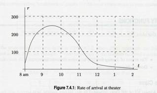
Here is the graph of the rate (in arrivals per hour) at which patrons arrive at the theater to get rush seats for the evening performance. The first people arrive at 8 a.m. and the ticket windows open at 9 a.m. Suppose that once the windows open, people can be served at an average rate of 200 per hour. Use the graph to approximate:
1) The length of the line at 9 a.m. when the windows open.
2) The length of the line at 10 a.m. and 11 a.m.
3) The rate at which the line is growing at 10 a.m.
4) The time when the line is longest.
5) The length of time a person who arrives at 9 a.m. has to stand in line.
6) The time the line disappears.
7) Suppose you were given a formula for r in terms of t. Explain how you would answer the above.
Activity 3: Balloon
flight.
Problem 38 page 262.
Goals: Using
the Fundamental Theorem of Calculus in real world settings.
Skills:
•
Know the Fundamental Theorem of Calculus. The
Fundamental Theorem of Calculus relates integral and derivative as
inverses. To find the integral, we
use the derivative, but for a function we might not yet know. Fortunately, the integral can be
interpreted as an area, so we don't need to know the original function explicitly
if we can approximate it using areas.
•
Be able to approximate areas under curves using
graphs. In the examples today we calculated areas given
graphs. This is usually best
accomplished with a suitable grid on graph paper, and counting boxes. But if other approximations work (like
triangles) you should use them.
The important part is being able to find a good answer for how much area
is bounded by the curve. Later
(Chapter 7) we will focus more on formulas.
Reading: Sections 6.1 and 6.2.
Activity: Examples using integrals. Quiz 7 today.
We will look at two examples today, one a general use of integrals and one from economics.
If we could replace a function over an interval with a constant, so that the areas are equal, then we would have the average value over that interval. The key idea is that the areas are equal. Because a constant function makes a rectangular area, all we need to calculate average area is the width of the interval and the area (the definite integral). In Activity 1 you will practice this rephrasing.
The second example is in economics. Consumer surplus is the amount of money not spent that would have been spent at higher prices. This is different for each consumer, as there are many different "demand" levels. So, for each price level, we determine how much money was "saved" from the actual price versus the willing price, as determined by the demand curve, and total this over all prices (down to the current price). Similarly, we can figure a producer surplus, but using the supply curve. Again the reasoning is that if the price were lower, fewer items would be made, and therefore sold. It is important to note that at equilibrium, both producers and consumers are "gaining" from the transaction.
Geometrically, the consumer surplus is the area bounded by the price (horizontal line) and the demand curve (integral area if the demand curve isn't linear). The producer surplus is the area below the price line bounded by the supply curve.
The interesting work comes when we (perhaps the government) impose non-equilibrium prices. What effect does this have on the economic interpretations? We will explore this idea in Activity 2. In class, I will work on Problem 10 page 285.
Activity 1: Average
Value.
Is the average of the maximum and minimum over an interval equal to the average value over the interval? Work Problems 12 and 18 on page 279, which address this.
Activity 2: Consumer
and Producer surplus.
Problem 9, page 285. I recommend graphing the curves in addition to using fnInt(.
Now suppose a price greater than equilibrium is imposed. (Invent one.) Calculate the change in the two surpluses.
Now suppose a price lower than equilibrium is imposed. (Invent one.) Calculate the change in the two surpluses.
Goals: Use
integrals in economics settings.
Skills:
•
Know the Average Value of a function over an interval. Graphically,
we can interpret the definite integral as the area of a rectangle over an
interval. The height of this
rectangle represents the average value of the function over the interval.
•
Understand the Consumer and Produce Surplus examples. Equilibrium
price is lower than many consumers are willing to pay. The difference between what they would have paid and what they are paying is called the consumer surplus. Similarly, the equilibrium price is
higher than many producers are willing to produce. The difference in the equilibrium price and the supplier's
willing price is the producer surplus.
Reading: Sections 7.1 and 7.2.
Activity: Antiderivatives. Integration by Substitution. Homework 7 due today.
We have explored how to interpret definite integrals. The techniques we've been using involve estimating areas under curves. The Fundamental Theorem of Calculus guided us, but it also shows us another approach to the solution, if we have a formula for the rate function (the derivative). The FTC says all we have to do is come up with a formula whose derivative is the formula we've started with. This sounds easier than it often is. In fact, there are some simple examples on page 304 for which no simple answer exists.
However, when such a formula does exist, the solution to a definite integral is then simply the difference of two values in this new function, which, because it is an inverse function, is called an antiderivative. It is important to note right away that antiderivatives are not unique functions. We know from Chapter 3 that when we add a constant to a function we don't change the derivative at all. So there are many antiderivatives to any problem, but they only differ by adding a different constant.
To find antiderivatives we need to recognize a few features of the rules we learned in Chapter 3. First, derivatives add together, so we can work on each part in a sum separately. Second, derivatives of power functions are themselves power functions. So we just need to work backwards. Exponential functions are also their own derivatives. Composed functions are another matter. They may or may not have simple solutions. We will use substitution to see if we can discover the answers to them.
Substitution doesn't always work; we have
to have functions that match the chain rule exactly. But substitution gives us a chance at least. It might require trial and error to
find the right substitution to make.
The strategy is to try w as an
"inner" function; then ![]() . Replacing what
we can, we see if we have made the problem into something simpler and
solvable. I will work problems in
class to show you the gist of it.
Then you will practice with both the simple functions (Activity 1) and
the composed functions (Activity 2).
. Replacing what
we can, we see if we have made the problem into something simpler and
solvable. I will work problems in
class to show you the gist of it.
Then you will practice with both the simple functions (Activity 1) and
the composed functions (Activity 2).
Activity 1: Working
"backwards".
Work as many of the problems on page 304 as you can.
Activity 2:
Integration by Substitution.
Work as many of the problems on page 308 as you can.
Goals: Realize
that antiderivatives are the inverses of derivatives. Know how to do integration by substitution.
Skills:
•
Realize that an antiderivative is a function whose
derivative is the original expression.
The Fundamental Theorem of Calculus
shows us that accumulated change in a function is an area under the derivative
curve. Conversely, if we know the
original function's formula, we can simply subtract two values to find the
definite integral.
•
Know how to find antiderivatives of simple functions. Power
functions, exponential functions, constants, and the reciprocal function 1/x
are all simple functions that have simple antiderivatives. Section 7.1 enumerates them in the
various boxed formulas.
•
Know how to find antiderivatives using substitution. The
antiderivatives for composed functions can sometimes be found using
substitution. This technique only
works if the derivative of the proposed substitution appears in the formula in
just the right way. If the
substitution is chosen well, then the problem after substitution will be of a
simpler nature.
Reading: Sections 7.3 and 7.4.
Activity: Analyzing Antiderivatives. Quiz 8 today.
Definite integrals, as we have seen, are specific areas under a curve. If we have a formula for the derivative that we can find an antiderivative for, we can use the Fundamental Theorem of Calculus to find the area exactly. Today we will do work very similar to yesterday's work, but we will move on to do the actual subtractions specified by the FTC.
In addition to finite integrals, we can
also try our hand at improper integrals,
or those with infinity in either integrand. These problems will be solved with limits, and therefore may
be tricky to conclude convergence with (recall the harmonic series of Day
1). However, the FTC saves us, if
we are able to evaluate the antiderivative as x approaches
infinity.
We will also revisit an activity from Chapter 2 (Day 9), and notice (hopefully) how much simpler the last part is now that we know about integration.
Activity 1:
Evaluating definite integrals exactly using the FTC.
For each of the following functions, find an antiderivative. Then, evaluate the definite integral using your calculator (fnInt), and by using the Fundamental Theorem of Calculus. Compare answers. Which one is "right" and which one is only an approximation?
1) ![]() . Integrate from
0 to 10.
. Integrate from
0 to 10.
2) ![]() . Note: you will
have to decide how to "con" your calculator into doing infinity.
. Note: you will
have to decide how to "con" your calculator into doing infinity.
3) ![]() . This integral
is one way to prove that the harmonic series diverges.
. This integral
is one way to prove that the harmonic series diverges.
Activity 2:
Estimating the derivative using a graph, and translating back.
Our next activity is a repeat of what we did on Day 9. It will take less time than before, hopefully.
Each of you will sketch an arbitrary function on a piece of paper, labeling it "Original Curve" and putting your name on it. You will then pass your graph to someone else; they will graph the derivative function on a separate sheet of paper, labeled with "Derivative Curve for <insert name here>". The person drawing the derivative will have to carefully estimate the slopes, so a scale is needed. Finally, the second person will pass the derivative graph to a third person (keep the original aside to compare with later); the third person will attempt to redraw the original graph based solely on the information from the derivative graph. Caution: this last part is tricky.
Note that the last part isn't nearly as tricky now as it was on Day 9; we now have the FTC to guide us in exactly how much to make the original graph rise or fall.
Goals: Calculate and interpret integrals using
antiderivatives.
Skills:
•
Evaluate definite integrals using both antiderivatives and
the TI-83. The definite integral can be calculated with
antiderivatives (using the Fundamental Theorem of Calculus) or by numerical
methods (using fnInt
on the TI-83). You can also use CALC 7 (∫f(x)dx) on the graphing window.
•
Be able to draw an antiderivative given a derivative
graph. On Day 9 it was difficult during our exercise to reconstruct the
original function from the derivative graph, because we didn't know how much to
increase or decrease the function just knowing the derivative. Now, after studying the FTC, we know
the area is the important
missing factor. With this
knowledge, you should now be able to draw accurate antiderivatives, as this is really what they are.
•
Be able to calculate an improper integral. An
improper integral involves infinity as one of the integrands. Therefore, to evaluate an improper
integral exactly, we must use the FTC and some limit ideas.
Reading: Sections 9.1 and 9.2.
Activity: Introduction to Multivariate Functions. Homework 8 due today.
The real world is rarely explained by
simple one-variable functions.
Everything depends on everything else. The complexity is sometimes daunting. However, we can try to model things
with mathematical formulas, and these often prove useful. For example, we know that the amount of
money in a bank account can be represented by the formula ![]() . We can view B as a function of three variables: P, r,
and t. Of course, in the real world the account balance won't
always be predicted by this formula unless the account is left completely
alone, and the bank doesn't close the account. In Activity 1, we will explore how to describe a
multi-variable function with a table.
. We can view B as a function of three variables: P, r,
and t. Of course, in the real world the account balance won't
always be predicted by this formula unless the account is left completely
alone, and the bank doesn't close the account. In Activity 1, we will explore how to describe a
multi-variable function with a table.
Graphically, we view multivariate
functions by holding all but two variables constant, and then graphing the
remaining two variables using plotting techniques we already know. Because we view the dependent variable
differently than the independent variables, the techniques fall into two basic
types.
Cross-sections occur when the dependent
variable is one of the two variables we graph. In a three-dimensional setting, we can imagine we have
"sliced" the surface vertically and are looking at the surface from the side,
in a cross-section. If we line up
a series of cross-sections, we may be able to visualize the three-dimensional
surface accurately. Cross-sections
can be done from any dimension, as long as the dependent variable is on the
vertical axis. Activity 2 today
will give us some practice with graphing cross-sections.
Contours occur in a three-dimensional
surface when the dependent variable is held constant, and the other two
variables are graphed. Due to the
nature of functions, cross-sections will always create graphable formulas, but
contours may result in something quite difficult to create. For example, it's not at all clear when
we begin what values to use for the dependent variable. Common uses for contours are maps. You have seen weather maps that
highlight temperatures. Instead of
simply showing the isotherms (lines of equal temperatures) color is commonly
used. In Activity 3 today we will
explore contours in more detail.
After you work on the three activities
today, I will explore ![]() . This function
is tougher than the one you're working on, but we should see all the same
issues.
. This function
is tougher than the one you're working on, but we should see all the same
issues.
Activity 1:
Describing a multivariate function with a table.
In your groups, create
tables of values for this two-variable function: ![]() . The goal is to
convey to a reader what the various values of B might be. I will let each
group decide how to make the table; we will compare among groups to see if you
chose similar methods.
. The goal is to
convey to a reader what the various values of B might be. I will let each
group decide how to make the table; we will compare among groups to see if you
chose similar methods.
Is B an increasing or a decreasing function?
Activity 2:
Describing a multivariate function with cross-sections.
Using ![]() hold P constant (choose some values) and draw the resulting
B vs. t graphs.
Then repeat holding t
constant and drawing the B vs. P graphs.
Do they give you the same impression of the surface? Is it the same as the impression you
got in Activity 1?
hold P constant (choose some values) and draw the resulting
B vs. t graphs.
Then repeat holding t
constant and drawing the B vs. P graphs.
Do they give you the same impression of the surface? Is it the same as the impression you
got in Activity 1?
Activity 3:
Describing a multivariate function with contours.
In practice, you will
most likely not be producing contours.
More often you will interpret them. But we want to be able to produce contours for simpler
functions. Again, using ![]() , create some contours.
You will need to choose some values of B to make the contours for.
It is not always clear what values will make the most sense. Trial and error may be in order. Does this contour graph give you the
same impression that you got in Activities 1 and 2?
, create some contours.
You will need to choose some values of B to make the contours for.
It is not always clear what values will make the most sense. Trial and error may be in order. Does this contour graph give you the
same impression that you got in Activities 1 and 2?
When graphing
cross-sections or contours, we may want to graph a whole series of values for x, or z. In our calculators, we can replace the
variable with a list that will accomplish this for us, saving a lot of
typing. For example, if we wanted
to graph ![]() for z = -20, -10, 0, 10, and 20, we can enter this: Y1={-20,-10,0,10,20}^2-x-3. The calculator will graph first
for z = -20, -10, 0, 10, and 20, we can enter this: Y1={-20,-10,0,10,20}^2-x-3. The calculator will graph first ![]() , then
, then ![]() , etc. One
drawback to this approach is that when you TRACE, you won't know which value in the list the
curve represents.
, etc. One
drawback to this approach is that when you TRACE, you won't know which value in the list the
curve represents.
Goals: Introduce
multivariate functions. Explore
tables, cross-sections, and contours as ways to view multivariate functions.
Skills:
•
Understand how to represent a multivariate function with a table of values. Tables
can describe multivariate functions, but they are not as good as graphs. On the other hand, graphs can be
difficult to produce or interpret, and sometimes having the raw numbers is
better. The best approach is to
have a formula, but many real world settings don't yield known formulas (daily
highs across the country is one example).
•
Be able to produce cross-sections for a multivariate
function. To make a cross-section of a multivariate function,
hold all but one of the independent variables constant; then graph the
dependent variable versus that last independent variable. Naturally, if there are many independent
variables held constant, it will be difficult to visualize the entire
surface. In the three-dimensional
case, we can think of this approach as vertical "slices" of the surface, viewed
from the side.
•
Be able to read and interpret contours for a multivariate
function. Contour diagrams are views from above,
basically. Imagine looking down on
the surface, in the case of three dimensions. Contours represent horizontal "slices". Contours may be difficult to produce,
as the curves traced out may not be functions at all (for example: circles at a
relative maximum).
Reading: Sections 9.3 and 9.4.
Activity: Calculating Partial Derivatives.
Just as for one-variable functions, we can talk about derivatives with multivariate functions. Basically, we will let one of the variables remain constant and explore how the other variable changes. This technique is called partial derivatives. All that we know about derivatives from earlier chapters apply here. One new aspect is that there are several possible derivatives. We also use different notations (see page 361).
There is another new idea about derivatives that we haven't encountered before: the mixed second partial derivative. The regular second partial derivatives measure concavity, the same as the one-variable second derivatives. But when we take the mixed second partial derivative (see page 370) we are really estimating how the change in one direction changes as we move in the other direction. We are more estimating a kind of "twisting" in the surface. We will make more use of this on Day 26 when we classify the extrema.
Activity 1:
Calculate partial derivatives from tabular data.
Problem 8 page 366.
Activity 2:
Calculate partial derivatives from graphs, both cross-sections and contours.
Using your graphs from ![]() from Activities
2 and 3 on Day 24, estimate some values of the partial derivatives.
from Activities
2 and 3 on Day 24, estimate some values of the partial derivatives.
Activity 3:
Calculate partial derivative formulas.
Verify your answers in Activity 2 using algebra. Then work on a few of problems 26 to 37 on page 372.
Goals: Calculate
partial derivatives from tabular data, from graphs (both cross-sections and
contours), and from formulas.
Skills:
•
Be able to estimate partial derivatives from tabular
data. Calculating a derivative from a table in two or more dimensions is no
different than it was in Chapter 2.
We use slopes of secant lines, and due to the nature of tabular data, we
can only "zoom in" so much. The
only trick is to pay attention to which variable is being held constant.
•
Be able to estimate partial derivatives from graphs. From
cross-section graphs, we can estimate the partial derivative for that variable
in just the same way as in Chapters 2 and 3. For the contour graphs, we must use a different approach. Typically, we will estimate the
difference between two contours, and express the ratio of the change in
contours to distance between contours as the derivative in that direction.
•
Be able to calculate partial derivatives from
formulas. Using the formulas from Chapter 4, we can calculate
partial derivatives exactly. The
only difficulty is keeping track of which variable is allowed to vary; our
notation is intended to remind us of this (see page 361).
Reading: Section 9.5.
Activity: Multivariate Optimization. Quiz 9 today.
To maximize or minimize a multivariate function, we use the same criteria we did for one-variable function: critical points and the second derivative test. The details are slightly different for the second derivative test, and we will do several problems today practicing this technique. First we solve the first derivatives jointly by setting them to zero. This will give us candidates for extrema. Now we use the second derivative test (page 376) to help classify the candidates as maxima, minima, or neither. It is also possible the test is inconclusive. In those situations, we must use some other approach, perhaps something akin to the first derivative test, although using that approach is a bit trickier in multiple dimensions. Note: solving the first derivative formulas simultaneously for all variables present may be very difficult. One special case is when all the derivatives are linear. Then you can use techniques from MATH 204 (the linear algebra/matrix results).
In addition to using formulas, make sure you can use graphs also to find extrema. Problems 1 and 2, and 14 to 16 on page 377 are good practice. A new sort of critical point occurs in multiple dimensions called a saddle point. You can think of a mountain pass as one example; in one direction (going over the pass) the function is a maximum but in the other direction (going from one mountain to the other through the pass) the function is a minimum. The second derivative test will classify these saddle points as "neither".
Activity 1:
Optimizing multivariate functions.
I will work problems 3 and 6 in class. Try as many of the others as you can. Problems 3 through 12 page 377.
Goals: Understand
how the derivatives can be used to find the extrema in multivariate functions.
Skills:
•
Be able to find the extrema using a contour graph. Extrema
on contour graphs are represented with closed loops. To find whether they are maxima or minima entails paying
attention to the values of the contours around the points.
•
Be able to find extrema using algebra. Using
the second derivative test, you should be able to classify the extrema as
maxima, minima, or neither. In
some cases, the second derivative test is inconclusive.
•
Understand the saddle point in multivariate functions. In
one direction, a saddle point is a maximum, but in another direction it is a
minimum. If we are trying to
optimize a function, it is critical to know if our critical points are maxima,
minima, saddle points, ridges, etc.
Reading: Chapters 5, 6, 7, and 9.
Activity: Presentation
3. Homework 9 due today.
Pick one of these functions
(first come, first served): 1)![]() , 2)
, 2)![]() , 3)
, 3)![]() , 4)
, 4)![]() , 5)
, 5)![]() , 6)
, 6)![]() , 7)
, 7)![]() . Graph some
cross-sections, a contour graph, and classify the critical points. Show how your critical points appear in
each of your displays.
. Graph some
cross-sections, a contour graph, and classify the critical points. Show how your critical points appear in
each of your displays.
Reading: Chapters 5, 6, 7, and 9.
Activity: Exam
3.
This last exam covers integrals, including antiderivatives, and multivariate functions, Chapters 5, 6, 7, and 9. Some of the questions will be multiple choice. Others will require you to show your worked out solution.
Populations for the 50 states, DC, and the USA, by
decade.
(in thousands)
|
|
AL |
AK |
AZ |
AR |
CA |
CO |
CT |
DE |
DC |
FL |
GA |
HI |
ID |
IL |
IN |
IA |
KS |
KY |
|
1790 |
|
|
|
|
|
|
238 |
59 |
|
|
83 |
|
|
|
|
|
|
74 |
|
1800 |
1 |
|
|
|
|
|
251 |
64 |
8 |
|
163 |
|
|
|
6 |
|
|
221 |
|
1810 |
9 |
|
|
1 |
|
|
262 |
73 |
16 |
|
252 |
|
|
12 |
25 |
|
|
407 |
|
1820 |
128 |
|
|
14 |
|
|
275 |
73 |
23 |
|
341 |
|
|
55 |
147 |
|
|
564 |
|
1830 |
310 |
|
|
30 |
|
|
298 |
77 |
30 |
35 |
517 |
|
|
157 |
343 |
|
|
688 |
|
1840 |
591 |
|
|
98 |
|
|
310 |
78 |
34 |
54 |
691 |
|
|
476 |
686 |
43 |
|
780 |
|
1850 |
772 |
|
|
210 |
93 |
|
371 |
92 |
52 |
87 |
906 |
|
|
851 |
988 |
192 |
|
982 |
|
1860 |
964 |
|
|
435 |
380 |
34 |
460 |
112 |
75 |
140 |
1057 |
|
|
1712 |
1350 |
675 |
107 |
1156 |
|
1870 |
997 |
|
10 |
484 |
560 |
40 |
537 |
125 |
132 |
188 |
1184 |
|
15 |
2540 |
1680 |
1194 |
364 |
1321 |
|
1880 |
1263 |
33 |
40 |
803 |
865 |
194 |
623 |
147 |
178 |
269 |
1542 |
|
33 |
3078 |
1978 |
1625 |
996 |
1649 |
|
1890 |
1513 |
32 |
88 |
1128 |
1213 |
413 |
746 |
168 |
230 |
391 |
1837 |
|
89 |
3826 |
2192 |
1912 |
1428 |
1859 |
|
1900 |
1829 |
64 |
123 |
1312 |
1485 |
540 |
908 |
185 |
279 |
529 |
2216 |
154 |
162 |
4822 |
2516 |
2232 |
1470 |
2147 |
|
1910 |
2138 |
64 |
204 |
1574 |
2378 |
799 |
1115 |
202 |
331 |
753 |
2609 |
192 |
326 |
5639 |
2701 |
2225 |
1691 |
2290 |
|
1920 |
2348 |
55 |
334 |
1752 |
3427 |
940 |
1381 |
223 |
438 |
968 |
2896 |
256 |
432 |
6485 |
2930 |
2404 |
1769 |
2417 |
|
1930 |
2646 |
59 |
436 |
1854 |
5677 |
1036 |
1607 |
238 |
487 |
1468 |
2909 |
368 |
445 |
7631 |
3239 |
2471 |
1881 |
2615 |
|
1940 |
2833 |
73 |
499 |
1949 |
6907 |
1123 |
1709 |
267 |
663 |
1897 |
3124 |
423 |
525 |
7897 |
3428 |
2538 |
1801 |
2846 |
|
1950 |
3062 |
129 |
750 |
1910 |
10586 |
1325 |
2007 |
318 |
802 |
2771 |
3445 |
500 |
589 |
8712 |
3934 |
2621 |
1905 |
2945 |
|
1960 |
3267 |
226 |
1302 |
1786 |
15717 |
1754 |
2535 |
446 |
764 |
4952 |
3943 |
633 |
667 |
10081 |
4662 |
2758 |
2179 |
3038 |
|
1970 |
3444 |
303 |
1775 |
1923 |
19971 |
2210 |
3032 |
548 |
757 |
6791 |
4588 |
770 |
713 |
11110 |
5195 |
2825 |
2249 |
3221 |
|
1980 |
3894 |
402 |
2717 |
2286 |
23668 |
2890 |
3108 |
594 |
638 |
9747 |
5463 |
965 |
944 |
11427 |
5490 |
2914 |
2364 |
3660 |
|
1990 |
4040 |
550 |
3665 |
2351 |
29760 |
3294 |
3287 |
666 |
607 |
12938 |
6478 |
1108 |
1007 |
11430 |
5544 |
2777 |
2478 |
3685 |
|
2000 |
4447 |
627 |
5131 |
2673 |
33872 |
4301 |
3406 |
784 |
572 |
15982 |
8186 |
1294 |
1294 |
12419 |
6080 |
2926 |
2688 |
4042 |
|
|
LA |
ME |
MD |
MA |
MI |
MN |
MS |
MO |
MT |
NE |
NV |
NH |
NJ |
NM |
NY |
NC |
ND |
OH |
|
1790 |
|
97 |
320 |
379 |
|
|
|
|
|
|
|
142 |
184 |
|
340 |
394 |
|
|
|
1800 |
|
152 |
342 |
423 |
|
|
8 |
|
|
|
|
184 |
211 |
|
589 |
478 |
|
45 |
|
1810 |
77 |
229 |
381 |
472 |
5 |
|
31 |
20 |
|
|
|
214 |
246 |
|
959 |
556 |
|
231 |
|
1820 |
153 |
298 |
407 |
523 |
9 |
|
75 |
67 |
|
|
|
244 |
278 |
|
1373 |
639 |
|
581 |
|
1830 |
216 |
399 |
447 |
610 |
32 |
|
137 |
140 |
|
|
|
269 |
321 |
|
1919 |
736 |
|
938 |
|
1840 |
352 |
502 |
470 |
738 |
212 |
|
376 |
384 |
|
|
|
285 |
373 |
|
2429 |
753 |
|
1519 |
|
1850 |
518 |
583 |
583 |
995 |
398 |
6 |
607 |
682 |
|
|
|
318 |
490 |
62 |
3097 |
869 |
|
1980 |
|
1860 |
708 |
628 |
687 |
1231 |
749 |
172 |
791 |
1182 |
|
29 |
7 |
326 |
672 |
94 |
3881 |
993 |
|
2340 |
|
1870 |
727 |
627 |
781 |
1457 |
1184 |
440 |
828 |
1721 |
21 |
123 |
42 |
318 |
906 |
92 |
4383 |
1071 |
2 |
2665 |
|
1880 |
940 |
649 |
935 |
1783 |
1637 |
781 |
1132 |
2168 |
39 |
452 |
62 |
347 |
1131 |
120 |
5083 |
1400 |
37 |
3198 |
|
1890 |
1119 |
661 |
1042 |
2239 |
2094 |
1310 |
1290 |
2679 |
143 |
1063 |
47 |
377 |
1445 |
160 |
6003 |
1618 |
191 |
3672 |
|
1900 |
1382 |
694 |
1188 |
2805 |
2421 |
1751 |
1551 |
3107 |
243 |
1066 |
42 |
412 |
1884 |
195 |
7269 |
1894 |
319 |
4158 |
|
1910 |
1656 |
742 |
1295 |
3366 |
2810 |
2076 |
1797 |
3293 |
376 |
1192 |
82 |
431 |
2537 |
327 |
9114 |
2206 |
577 |
4767 |
|
1920 |
1799 |
768 |
1450 |
3852 |
3668 |
2387 |
1791 |
3404 |
549 |
1296 |
77 |
443 |
3156 |
360 |
10385 |
2559 |
647 |
5759 |
|
1930 |
2102 |
797 |
1632 |
4250 |
4842 |
2564 |
2010 |
3629 |
538 |
1378 |
91 |
465 |
4041 |
423 |
12588 |
3170 |
681 |
6647 |
|
1940 |
2364 |
847 |
1821 |
4317 |
5256 |
2792 |
2184 |
3785 |
559 |
1316 |
110 |
492 |
4160 |
532 |
13479 |
3572 |
642 |
6908 |
|
1950 |
2684 |
914 |
2343 |
4691 |
6372 |
2982 |
2179 |
3955 |
591 |
1326 |
160 |
533 |
4835 |
681 |
14830 |
4062 |
620 |
7947 |
|
1960 |
3257 |
969 |
3101 |
5149 |
7823 |
3414 |
2178 |
4320 |
675 |
1411 |
285 |
607 |
6067 |
951 |
16782 |
4556 |
632 |
9706 |
|
1970 |
3645 |
994 |
3924 |
5689 |
8882 |
3806 |
2217 |
4678 |
694 |
1485 |
489 |
738 |
7171 |
1017 |
18241 |
5084 |
618 |
10657 |
|
1980 |
4206 |
1125 |
4217 |
5737 |
9262 |
4076 |
2521 |
4917 |
787 |
1570 |
801 |
921 |
7365 |
1303 |
17558 |
5880 |
653 |
10798 |
|
1990 |
4220 |
1228 |
4781 |
6016 |
9295 |
4375 |
2573 |
5117 |
799 |
1578 |
1202 |
1109 |
7730 |
1515 |
17990 |
6629 |
639 |
10847 |
|
2000 |
4469 |
1275 |
5296 |
6349 |
9938 |
4919 |
2845 |
5595 |
902 |
1711 |
1998 |
1236 |
8414 |
1819 |
18976 |
8049 |
642 |
11353 |
|
|
OK |
OR |
PA |
RI |
SC |
SD |
TN |
TX |
UT |
VT |
VA |
WA |
WV |
WI |
WY |
USA |
|
1790 |
|
|
434 |
69 |
249 |
|
36 |
|
|
85 |
692 |
|
56 |
|
|
3929 |
|
1800 |
|
|
602 |
69 |
346 |
|
106 |
|
|
154 |
808 |
|
79 |
|
|
5308 |
|
1810 |
|
|
810 |
77 |
415 |
|
262 |
|
|
218 |
878 |
|
105 |
|
|
7240 |
|
1820 |
|
|
1049 |
83 |
503 |
|
423 |
|
|
236 |
938 |
|
137 |
|
|
9638 |
|
1830 |
|
|
1348 |
97 |
581 |
|
682 |
|
|
281 |
1044 |
|
177 |
|
|
12866 |
|
1840 |
|
|
1724 |
109 |
594 |
|
829 |
|
|
292 |
1025 |
|
225 |
31 |
|
17069 |
|
1850 |
|
12 |
2312 |
148 |
669 |
|
1003 |
213 |
11 |
314 |
1119 |
1 |
302 |
305 |
|
23192 |
|
1860 |
|
52 |
2906 |
175 |
704 |
5 |
1110 |
604 |
40 |
315 |
1220 |
12 |
377 |
776 |
|
31443 |
|
1870 |
|
91 |
3522 |
217 |
706 |
12 |
1259 |
819 |
87 |
331 |
1225 |
24 |
442 |
1055 |
9 |
38558 |
|
1880 |
|
175 |
4283 |
277 |
996 |
98 |
1542 |
1592 |
144 |
332 |
1513 |
75 |
618 |
1315 |
21 |
50189 |
|
1890 |
259 |
318 |
5258 |
346 |
1151 |
349 |
1768 |
2236 |
211 |
332 |
1656 |
357 |
763 |
1693 |
63 |
62980 |
|
1900 |
790 |
414 |
6302 |
429 |
1340 |
402 |
2021 |
3049 |
277 |
344 |
1854 |
518 |
959 |
2069 |
93 |
76212 |
|
1910 |
1657 |
673 |
7665 |
543 |
1515 |
584 |
2185 |
3897 |
373 |
356 |
2062 |
1142 |
1221 |
2334 |
146 |
92228 |
|
1920 |
2028 |
783 |
8720 |
604 |
1684 |
637 |
2338 |
4663 |
449 |
352 |
2309 |
1357 |
1464 |
2632 |
194 |
106022 |
|
1930 |
2396 |
954 |
9631 |
687 |
1739 |
693 |
2617 |
5825 |
508 |
360 |
2422 |
1563 |
1729 |
2939 |
226 |
123203 |
|
1940 |
2336 |
1090 |
9900 |
713 |
1900 |
643 |
2916 |
6415 |
550 |
359 |
2678 |
1736 |
1902 |
3138 |
251 |
132165 |
|
1950 |
2233 |
1521 |
10498 |
792 |
2117 |
653 |
3292 |
7711 |
689 |
378 |
3319 |
2379 |
2006 |
3435 |
291 |
151326 |
|
1960 |
2328 |
1769 |
11319 |
859 |
2383 |
681 |
3567 |
9580 |
891 |
390 |
3967 |
2853 |
1860 |
3952 |
330 |
179323 |
|
1970 |
2559 |
2092 |
11801 |
950 |
2591 |
666 |
3926 |
11199 |
1059 |
445 |
4651 |
3413 |
1744 |
4418 |
332 |
203302 |
|
1980 |
3025 |
2633 |
11865 |
947 |
3121 |
691 |
4591 |
14226 |
1461 |
511 |
5347 |
4132 |
1950 |
4706 |
470 |
226542 |
|
1990 |
3146 |
2842 |
11882 |
1003 |
3487 |
696 |
4877 |
16987 |
1723 |
563 |
6187 |
4867 |
1793 |
4892 |
454 |
248710 |
|
2000 |
3451 |
3421 |
12281 |
1048 |
4012 |
755 |
5689 |
20852 |
2233 |
609 |
7079 |
5894 |
1808 |
5364 |
494 |
281422 |

Managed by chris
edwards:
click to email chris edwards
Last updated August 26, 2008